Custom-Built Lightweight Open-Source FastICA Algorithm for In-Browser Use
Custom-Built FastICA on PyScript Methodology, to Separate Mixed Heart and Lung Sounds
Log Console
ICA PyScript Example
Due to the limitations of Pyodide which does not include support for the librosa Python library, we will exclusively work with WAV files, specifically those with a sample rate of 44100 Hz. No other types of audio files will be considered.
Independent Component Analysis (ICA) Algorithm (primarily derived from the Book: "Independent Component Analysis, A Tutorial Introduction" by James V. Stone)
(A) Introduction to the Fundamentals of ICA: Distinguishing It from PCA
Independent Component Analysis (ICA) is a computational technique designed to separate a multivariate signal into its additive, independent non-Gaussian components. This method is particularly effective for analyzing mixed signals that originate from multiple sources. In contrast to Principal Component Analysis (PCA), which seeks orthogonal components that maximize variance under the assumption of Gaussian source signals, ICA identifies components based on their statistical independence rather than their variance. Unlike PCA, which is significantly influenced by the orientation of the first eigenvector, ICA does not prioritize components based on variance. Instead, it focuses on the statistical independence of components, ensuring that each component's amplitude at any given point is unrelated to that of any other at the same time, indicative of their origins from distinct physical processes.
PCA reduces data dimensionality by emphasizing the variance captured by the first few eigenvectors, potentially leading to a reliance on the first principal component. This reliance is due to the first eigenvector's orientation, determined by the direction associated with the maximum variance principal component (PC). In contrast, ICA's approach to signal separation is not constrained by the variance or order of components. It seeks to identify independent sources within the signal mixtures, guided by the statistical properties of the signals rather than their variance. This fundamental difference underlines ICA's utility in separating mixed signals into components that represent original, independent sources, free from the hierarchical constraints of variance prioritization seen in PCA.
(B) Mathematical Foundations and Properties of Signal Mixtures
ICA is rooted in fundamental mathematical concepts such as entropy maximization, likelihood estimation, and the utilization of non-linear functions, notably the hyperbolic tangent (tanh), to approximate the cumulative distribution functions (CDFs) of source signals. A hallmark of successful separation through ICA is the alignment of the joint distribution of signals with the product of their marginal distributions, signifying statistical independence. Key characteristics of signal mixtures include (1) the independence of source signals versus the dependence observed in mixtures, (2) the presence of non-Gaussian histograms for each source signal in contrast to Gaussian histograms for mixtures, and (3) the lower complexity found in the simplest source signal compared to any of its mixtures. These principles underscore the theoretical and practical underpinnings of ICA, distinguishing it from other signal processing methods by emphasizing the non-Gaussian nature and statistical independence of source signals.
(C) ICA Applications and Its Spatial-Temporal Versatility
Independent Component Analysis (ICA) boasts a wide array of applications, from speech processing and brain imaging using functional Magnetic Resonance Imaging (fMRI) to the analysis of electrical brain signals via Electroencephalography (EEG). Its core advantage lies in the ability to discern and isolate source signals from their mixtures based on unique properties — particularly their statistical independence, non-Gaussian distribution, and comparative simplicity. This distinction is crucial in fields requiring precise signal separation, such as distinguishing individual voices in a noisy environment or isolating specific brain activities from complex imaging data. Furthermore, ICA's adaptability is showcased through its spatial and temporal variants: Spatial ICA (sICA) excels in analyzing data points like image pixels to segregate different visual sources, making it indispensable in image processing, while Temporal ICA (tICA) is pivotal for unraveling sequences over time, such as isolating distinct audio tracks or analyzing temporal brain signal patterns. This dual capability highlights ICA's comprehensive approach to addressing analytical challenges across a spectrum of domains, enhancing its utility in both spatially and temporally oriented data analysis.
(D) Algorithmic Steps of ICA
Preliminary Steps: The preprocessing of signals is critical before optimizing the unmixing matrix for signal separation.
Centering: Each signal within the mixtures is centered by subtracting its mean. Centering ensures that the signals adhere to a zero-mean, which is a prerequisite for any linear transformation of data in ICA, akin to PCA.
Whitening: The process starts with the computation of the covariance matrix of the centered signals, followed by eigenvalue decomposition. The subsequent transformation, using the eigenvectors and eigenvalues, renders the signals uncorrelated with unit variance. Whitening is a pivotal step as it reduces the complexity of isolating independent components by converting the signals into a space where they are linearly uncorrelated. This mirrors the preprocessing in PCA but is tailored to meet the distinctive requirements of ICA, which is the facilitation of component independence.
Optimizing the Unmixing Matrix: This is the iterative core of ICA, where the unmixing matrix is refined to separate the mixed signals.
Estimating Independent Components: At each iteration, the whitened signals are transformed by the unmixing matrix to estimate the independent components. This is based on the ICA premise that signals are linear combinations of independent components, and the unmixing matrix is the key to reversing their mixture.
Non-linearity Application: The estimates are then processed through the non-linear function tanh. This crucial step injects non-Gaussianity into the model, a cornerstone of ICA, enabling the distinction of the independent components from the mixtures. This is in contrast to PCA, which operates under the Gaussianity assumption and does not factor in independence.
Updating the Unmixing Matrix: The update rule integrates the outcomes of the non-linear function and its derivative. This follows the gradient ascent strategy, aiming to maximize the non-Gaussianity and consequently, the independence of the estimated components. It is anchored in the statistical tenet that independent components are discoverable by maximizing entropy or, equivalently, minimizing mutual information.
Convergence and Extraction: The final steps involve confirming the independence of the components and extracting them.
Convergence Check: The iterative process persists until the adjustments in the unmixing matrix diminish below a pre-set threshold, signifying that the components' independence will not significantly improve with further matrix alterations. This step is crucial to prevent an endless loop and to ascertain that the components are as independent as practically attainable.
Extracting Independent Components: With an optimized unmixing matrix, it is applied to the whitened signals to derive the final independent components. This marks the ICA process's culmination, where the theoretical and statistical frameworks are realized by segregating the mixed signals into their independent elements.
(E) Characteristics of the FastICA Algorithm (Hyvärinen, A. & Oja, E. (2000). Neural Networks, 13(4-5), 411-430.)
FastICA, while aligned with the fundamental objective of the ICA to separate mixed signals into independent components, introduces specific nuances in its approach, theoretical focus, and practical execution, making it a variant of the broader family of ICA algorithms.
Distinctly, FastICA is tailored for rapid convergence by employing a negentropy approximation to optimize for non-Gaussianity. Its fixed-point iteration scheme for updating the unmixing matrix stands out for its efficiency. Although the implementation may slightly differ concerning the choice of non-linear functions (e.g., logcosh or exp) to approximate negentropy, the underlying principle of non-Gaussianity maximization remains intact. Other salient features include:
"Fixed-Point Iteration Scheme": Utilizing specific non-linear functions and their derivatives to enhance non-Gaussianity.
"Symmetric Decorrelation": Ensured within each iteration to preserve the orthogonality and thus independence of the separated components.
Efficient "Convergence" Criterion: Based on the alterations in the unmixing matrix, it guarantees the prompt conclusion of the algorithm post the adequate extraction of independent components.
(F) Innovative Uses of ICA in Enhancing Alexa's Sound Recognition and Interaction
Amazon's Alexa is equipped with an innovative feature through its LED ring atop the device, which plays a crucial role beyond mere aesthetic appeal. When activated with the wake word "Alexa," this LED ring serves as a directional indicator, illuminating to point towards the source of the voice. This functionality not only adds an element of interaction by mimicking human-like responsiveness to sound sources but also signifies the sophisticated audio processing capabilities of the device. The directional illumination of the LED ring is a direct outcome of the device's ability to analyze and locate the origin of the sound, a process rooted deeply in the principles of independent component analysis (ICA).
ICA is pivotal for two primary functions within Alexa's operational framework. Firstly, it aids in pinpointing the direction from which the voice command is issued. By separating the mixed audio signals received by Alexa's microphones into their independent components, the system can identify the specific direction of the sound source. This process allows Alexa to "focus" on the speaker, enhancing user interaction by providing visual feedback through the LED ring.
Secondly, ICA plays a vital role in background noise reduction, a critical factor in far-field speech recognition. Voice commands captured from a distance inherently carry more noise and reverberation compared to those spoken directly into a device, such as a smartphone. These disturbances, primarily caused by sound waves reflecting off surfaces like walls or windows, can significantly hinder speech recognition accuracy. Through ICA, Alexa can effectively isolate the voice command from the background noise and reverberation. This isolation not only improves the clarity of the signal being processed but also enhances Alexa's ability to understand and respond to the user accurately, even in acoustically challenging environments.
(G) Reference
Original FastICA academic paper: Hyvärinen, A., & Oja, E. (2000). Independent Component Analysis: Algorithms and Applications. Neural Networks, 13(4-5), 411-430. Neural Networks Research Centre, Helsinki University of Technology.
ICA Introduction book: Stone, J.V. (2004). Independent Component Analysis: A Tutorial Introduction. Bradford Books. ISBN 978-0262693158.
scikit-learn. (n.d.). FastICA. Retrieved from https://scikit-learn.org/stable/modules/generated/sklearn.decomposition.FastICA.html
CRAN. (n.d.). fastICA. Retrieved from https://cran.r-project.org/web/packages/fastICA/index.html
Convert MP3 to WAV on Mac and Linux
Since Python Pyscript does not support the use of the librosa or pydub libraries in a browser-based environment, it is recommended to convert MP3 files to WAV format before using this browser-based Pyscript code, if WAV files are not already available.
(A) Using ffmpeg
Mac: Install using Homebrew:
brew install ffmpeg
Linux: Install using apt for Ubuntu or Debian:
sudo apt-get install ffmpeg
Once ffmpeg is installed, you can convert an MP3 file to WAV format with the following command:
ffmpeg -i input.mp3 output.wav
(B) Using sox
Mac: Install using Homebrew:
brew install sox
Linux: Install using apt for Ubuntu or Debian:
sudo apt-get install sox
With sox installed, convert an MP3 file to WAV format with the following command:
sox input.mp3 output.wav
FastICA Python Source Code, PyPI Package, and Local Demo
Installable Python package: ngene-fastica
The custom-built FastICA source code shown below has also been published as an installable Python package,
ngene-fastica, for local waveform separation examples and educational biomedical signal-processing demonstrations.
This package is intended for users who would like to test the FastICA implementation locally without configuring
PyScript, browser-side audio handling, or JavaScript-based waveform controls.
Quick installation
python -m pip install ngene-fastica
Minimal Python example
import numpy as np
from ngene_fastica import FastICA

# Rows represent observed mixtures; columns represent time samples.
X = np.random.randn(3, 10000)

ica = FastICA(n_components=3, random_state=42)
S = ica.fit_transform(X)

print(S.shape)
Run the local waveform separation demo
ngene-fastica-demo
The local demo writes example WAV files for source signals, mixed signals, and separated signals.
Please note that ICA separation may recover components in a different order or sign, which is a normal property of ICA.
Use case
Recommended option
Purpose
Browser-based demonstration
This PyScript page
Interactive waveform separation and visual demonstration inside the browser
Local Python test
pip install ngene-fastica
Run the FastICA package locally without PyScript configuration
Algorithm review
nGeneFastICA.py
Read the commented source code and follow the algorithmic steps
Prototype Python Script: Heart and Lung Sound Separation with Scikit-learn's FastICA
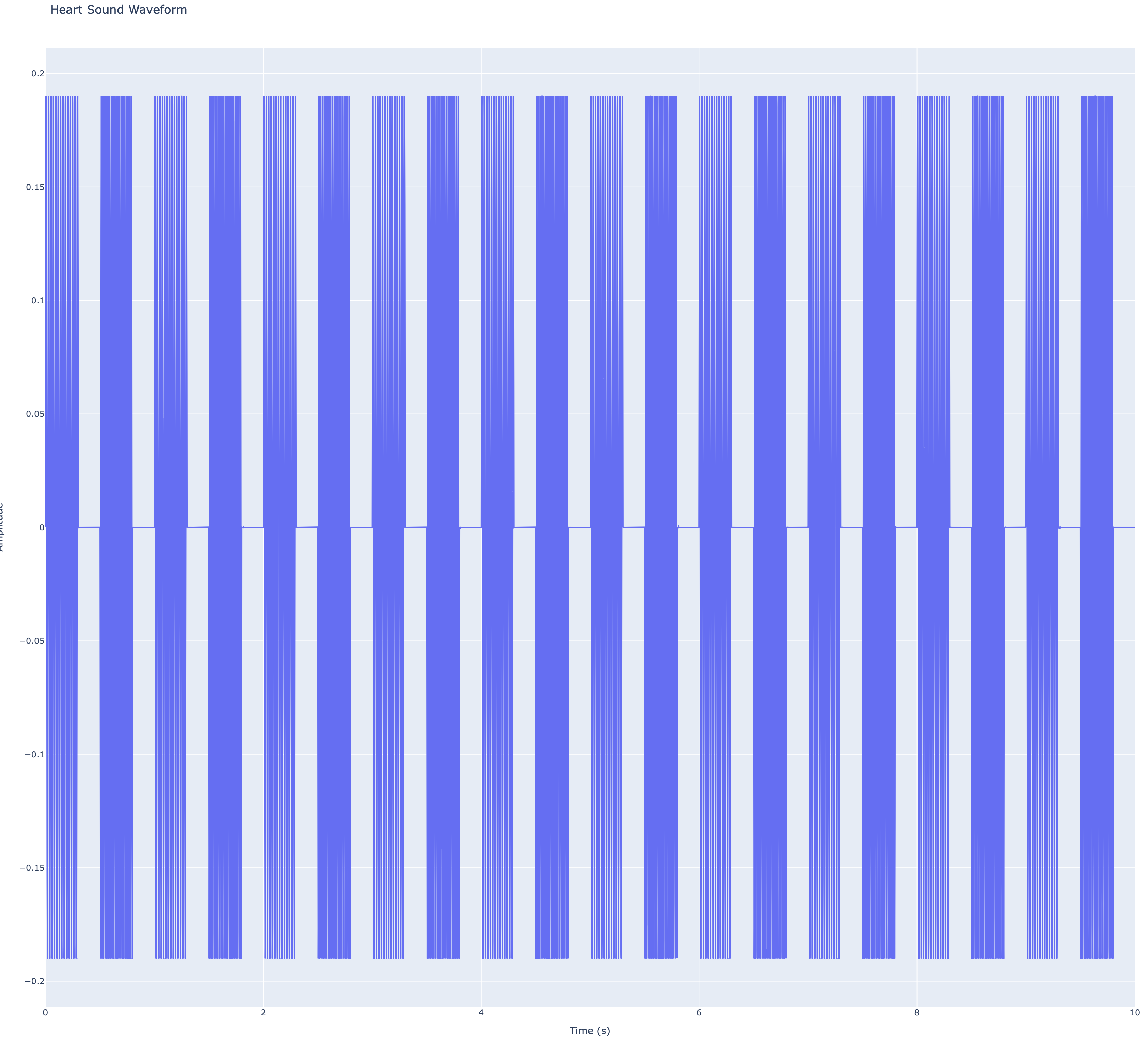
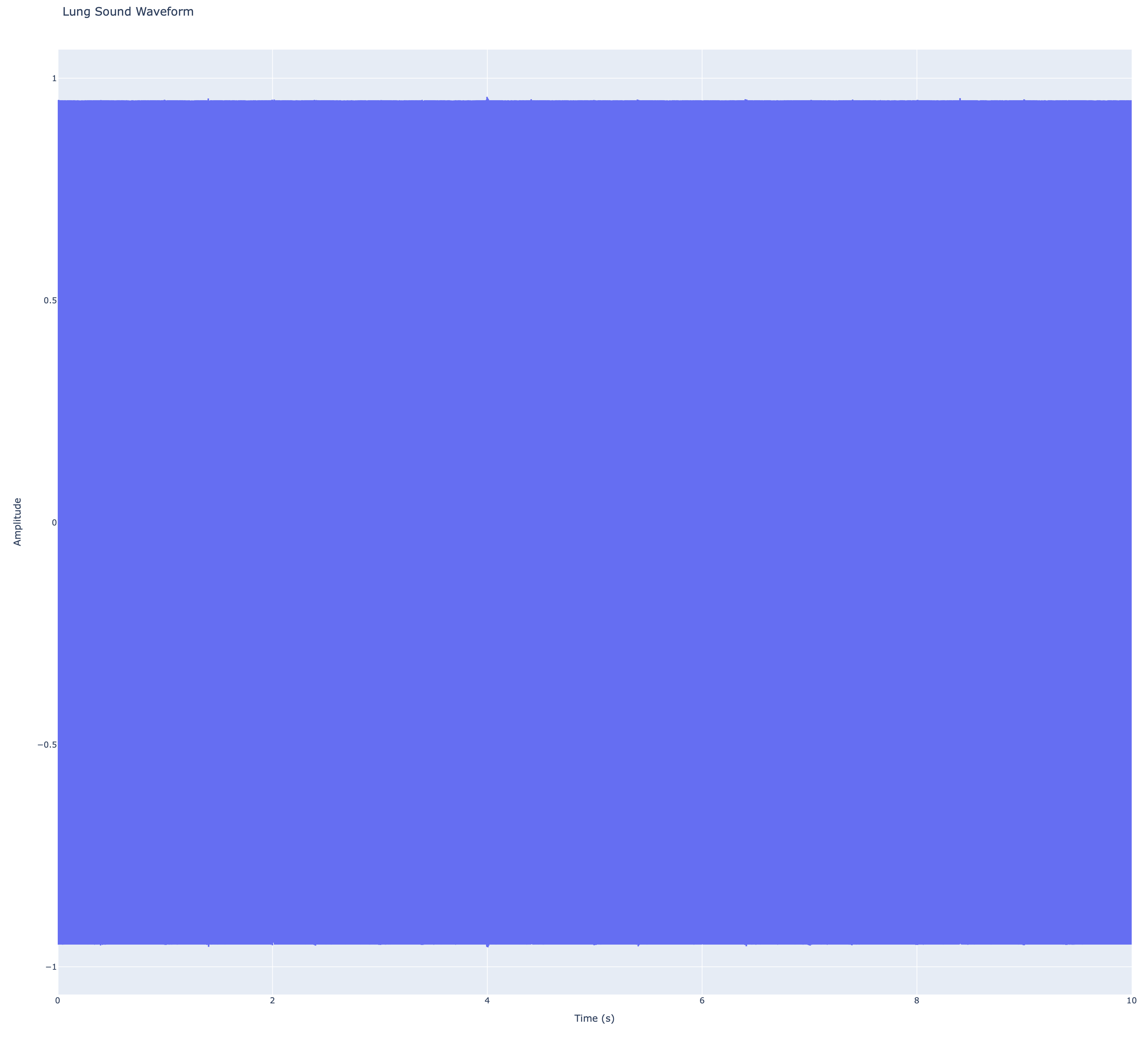
This explores the field of audio processing with our Independent Component Analysis (ICA) tool, crafted with medical professionals and researchers in mind. This software aids in the separation of complex audio signals, with a focus on heart and lung sounds.
Audio Signal Processing: Our tool expertly processes audio files, particularly heart and lung sounds, to analyze and separate these complex signals.
Display Waveforms: It visualizes the waveforms of these sounds, providing a clear, graphical representation of audio data.
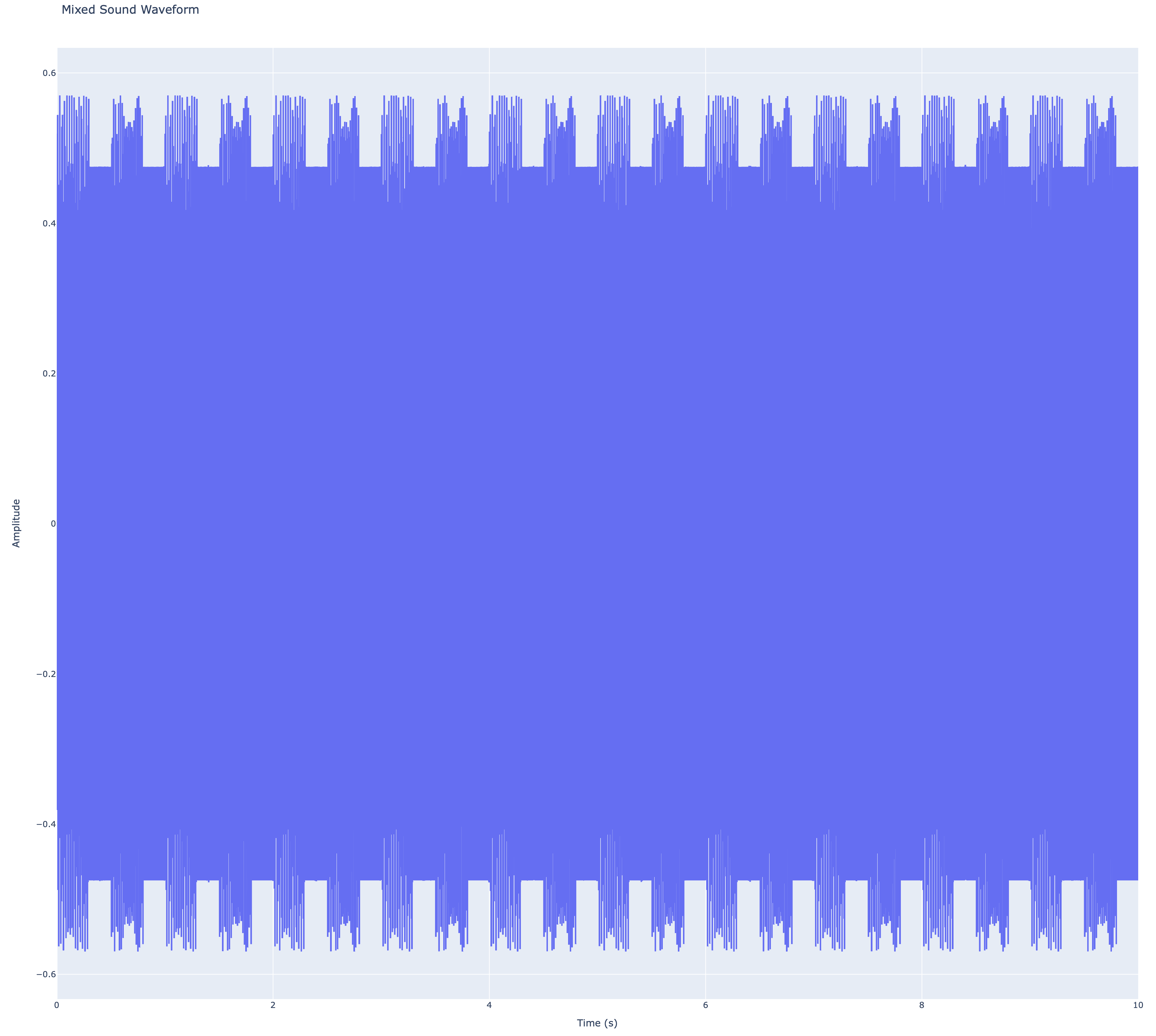
Merge Audio for Analysis: The software can merge two different audio signals for detailed analysis using ICA, ensuring comprehensive examination of overlapping sounds.
Independent Component Analysis: Utilizing ICA, the tool separates mixed audio signals into their individual components, allowing for in-depth analysis of each signal.
Audio Saving Capabilities: It offers functionality to save the separated audio components in both MP3 and WAV formats for further use and examination.
Direct Integration of R Scripts in Python: Executing FastICA.R for Signal Separation
In the pursuit of advancing and streamlining signal processing workflows, two new Python modules have been developed: nGene_rpy2 and nGene_Waveform. These modules are designed to facilitate the integration of R scripts into Python applications and to efficiently manage waveform data. The following sections provide an overview of these modules and demonstrate their practical applications.
(A) nGene_rpy2: Bridging R and Python
nGene_rpy2 is a Python class that utilizes the rpy2 library to seamlessly integrate R scripts and packages into Python applications. This class enables the loading of R code from files or strings, the importation of R packages, and the invocation of R functions directly from Python. Such integration is instrumental in leveraging R's advanced statistical and signal processing capabilities within a Python environment.
Load R Scripts: Facilitates the loading of R code from files or strings, creating callable modules within Python.
Import R Packages: Manages the importation of R packages, including automatic installation if packages are not already present.
Call R Functions: Executes R functions from loaded scripts or packages with automatic data conversion between R and Python data structures.
Execute R Commands: Allows the execution of raw R commands directly from Python, providing flexibility in scripting.
The following example demonstrates the utilization of nGene_rpy2 to perform Independent Component Analysis (ICA) using R's fastICA function:
nGene_Waveform is a Python class dedicated to the processing and visualization of waveform data. This class simplifies tasks such as reading audio files, normalizing signals, saving audio data, and plotting waveforms. It is essential for applications involving audio signal processing, particularly within the context of biomedical signals like heart and lung sounds.
Read and Normalize Audio Data: Facilitates the loading of .wav files and normalization of audio signals for processing.
Save Audio Signals: Enables the saving of processed or separated signals as .wav files.
Plot Waveforms: Provides visualization of audio signals using matplotlib for analysis and presentation purposes.
Handle Multiple Signals: Efficiently manages and processes multiple audio signals or components.
The example below illustrates how to utilize nGene_Waveform to read audio files and plot their waveforms:
main.py serves as an example script demonstrating the application of the nGene_rpy2 and nGene_Waveform classes to perform Independent Component Analysis (ICA) on mixed audio signals, such as heart and lung sounds. Users may adapt this script to their specific requirements by renaming it accordingly.
Initialize Handlers: Establishes instances of nGene_rpy2 and nGene_Waveform.
Load and Normalize Audio Data: Reads heart and lung sound files and normalizes the signals.
Mix Signals: Combines the original signals using a predefined mixing matrix.
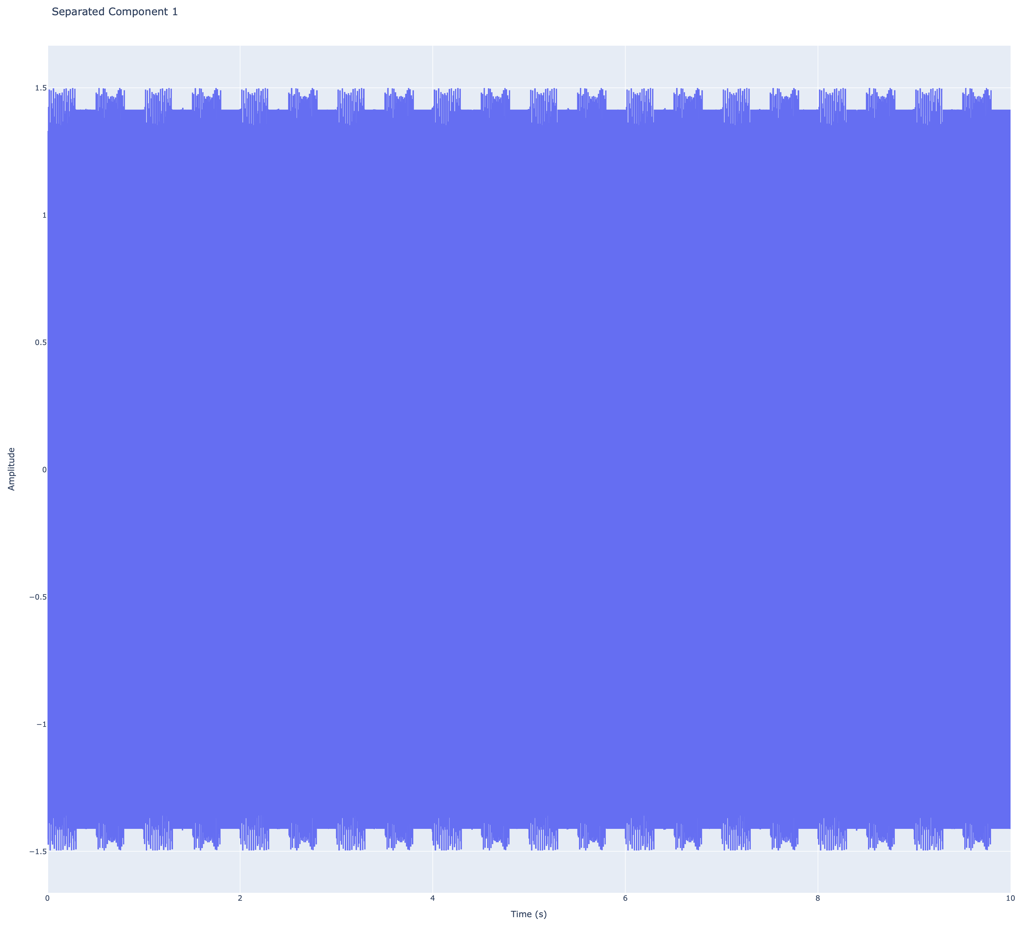
Perform ICA: Utilizes R's fastICA function to separate the mixed signals into independent components.
Plot and Save Results: Visualizes the original, mixed, and separated signals, and saves the separated components as .wav files.
The complete script is available in main.py. Users may adapt this script as needed:
Initialize Handlers:
Import and instantiate nGene_rpy2 and nGene_Waveform.
Load the R script for fastICA using nGene_rpy2.
Load and Normalize Audio Data:
Use nGene_Waveform to read and normalize heart and lung sound files.
Ensure both audio files have matching sample rates.
Mix Signals:
Combine the original signals using a predefined mixing matrix to create mixed signals.
Perform ICA:
Employ nGene_rpy2 to execute the fastICA function from R on the mixed signals.
Extract the separated independent components from the ICA result.
Plot and Save Results:
Visualize the original, mixed, and separated signals using nGene_Waveform.
Save the separated components as .wav files for further analysis or playback.
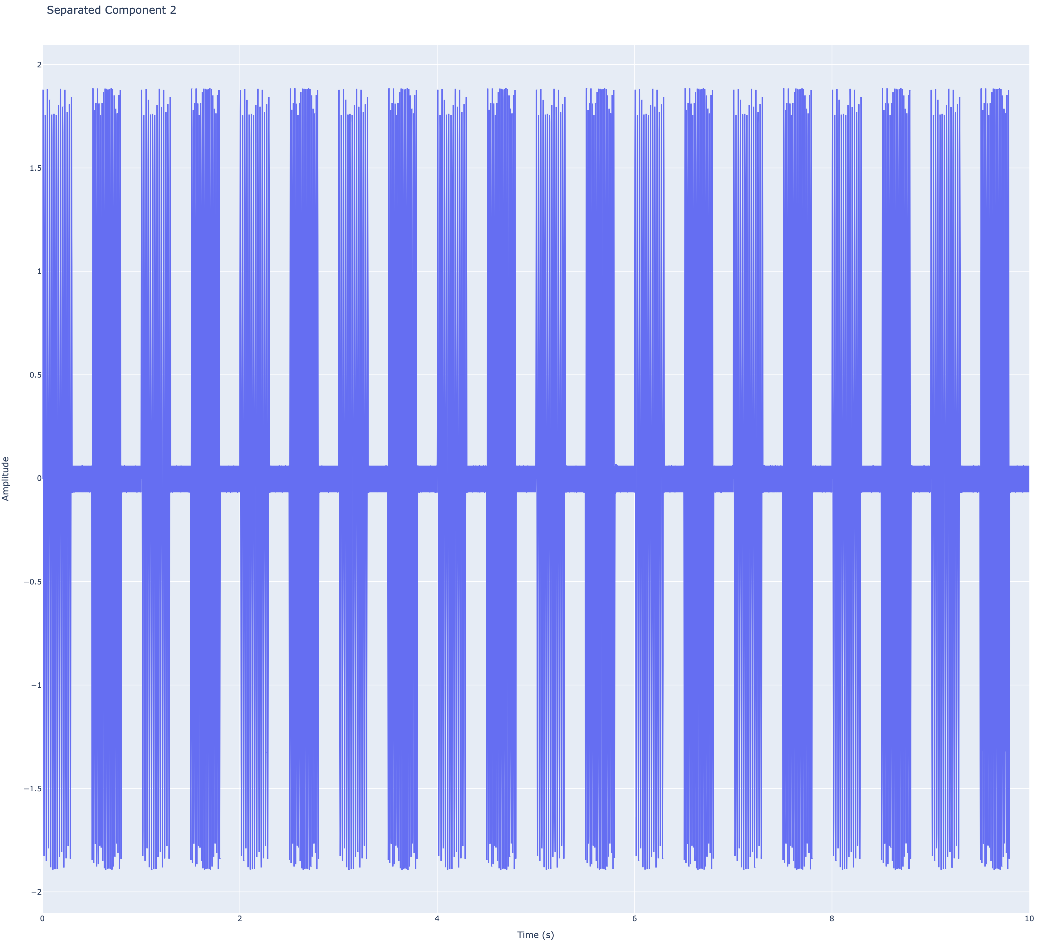
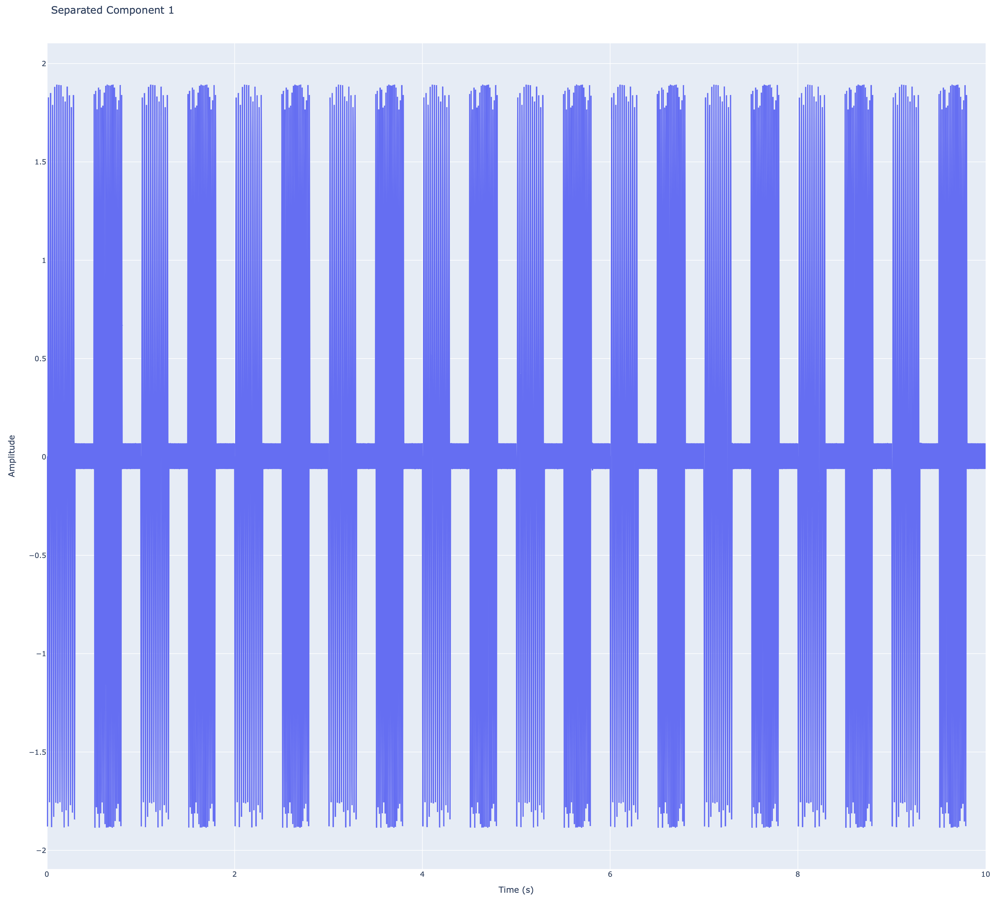
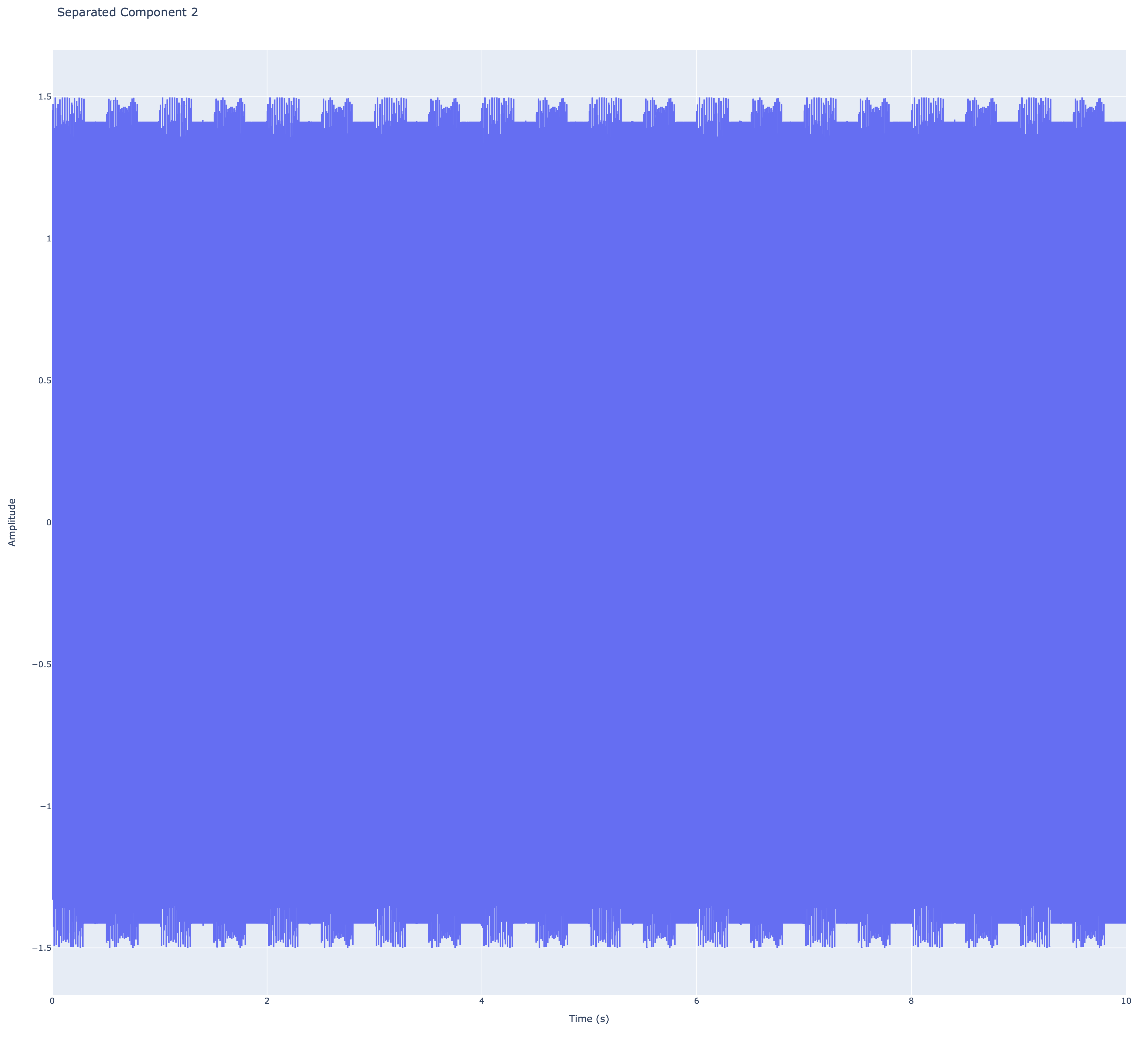
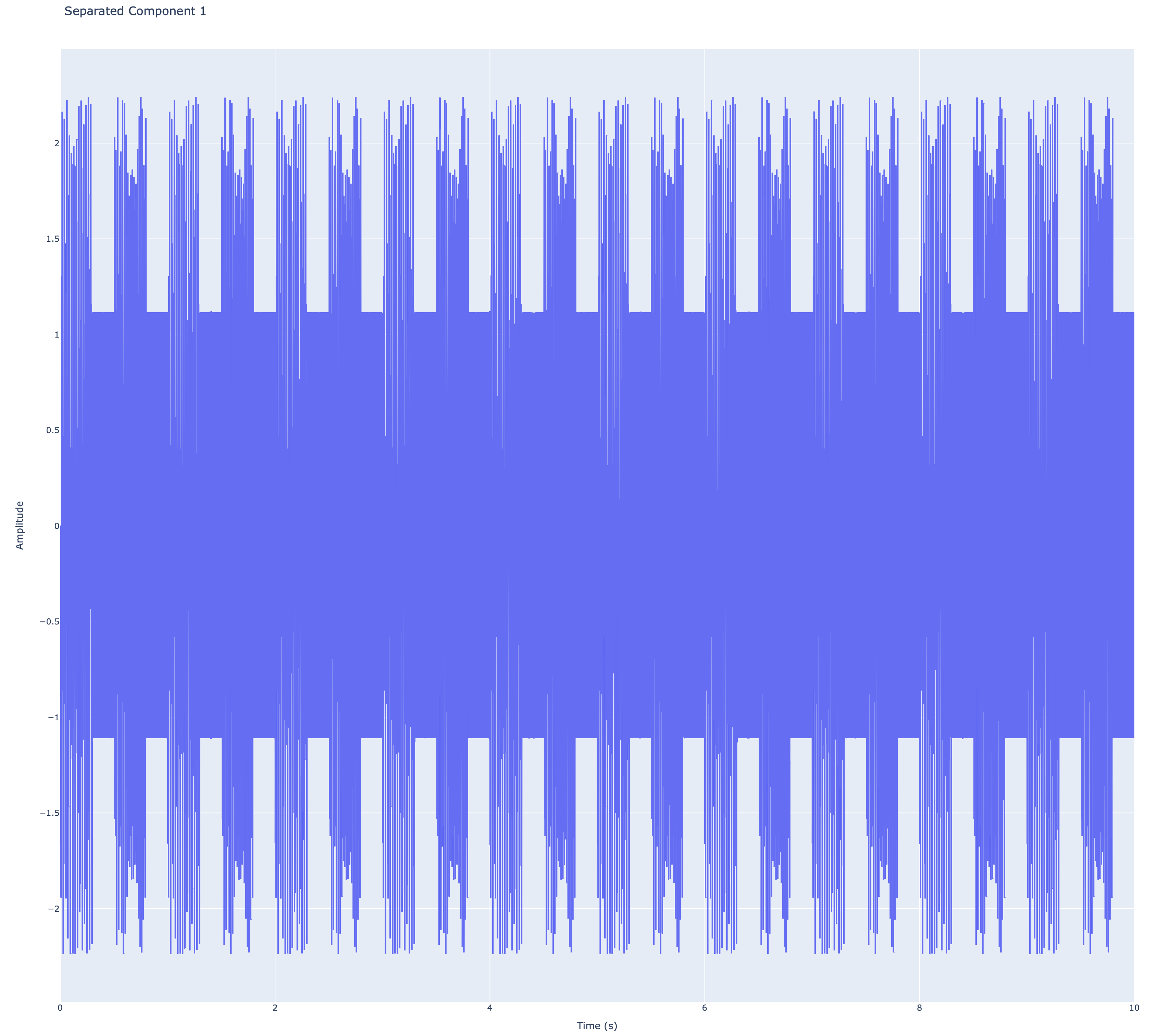
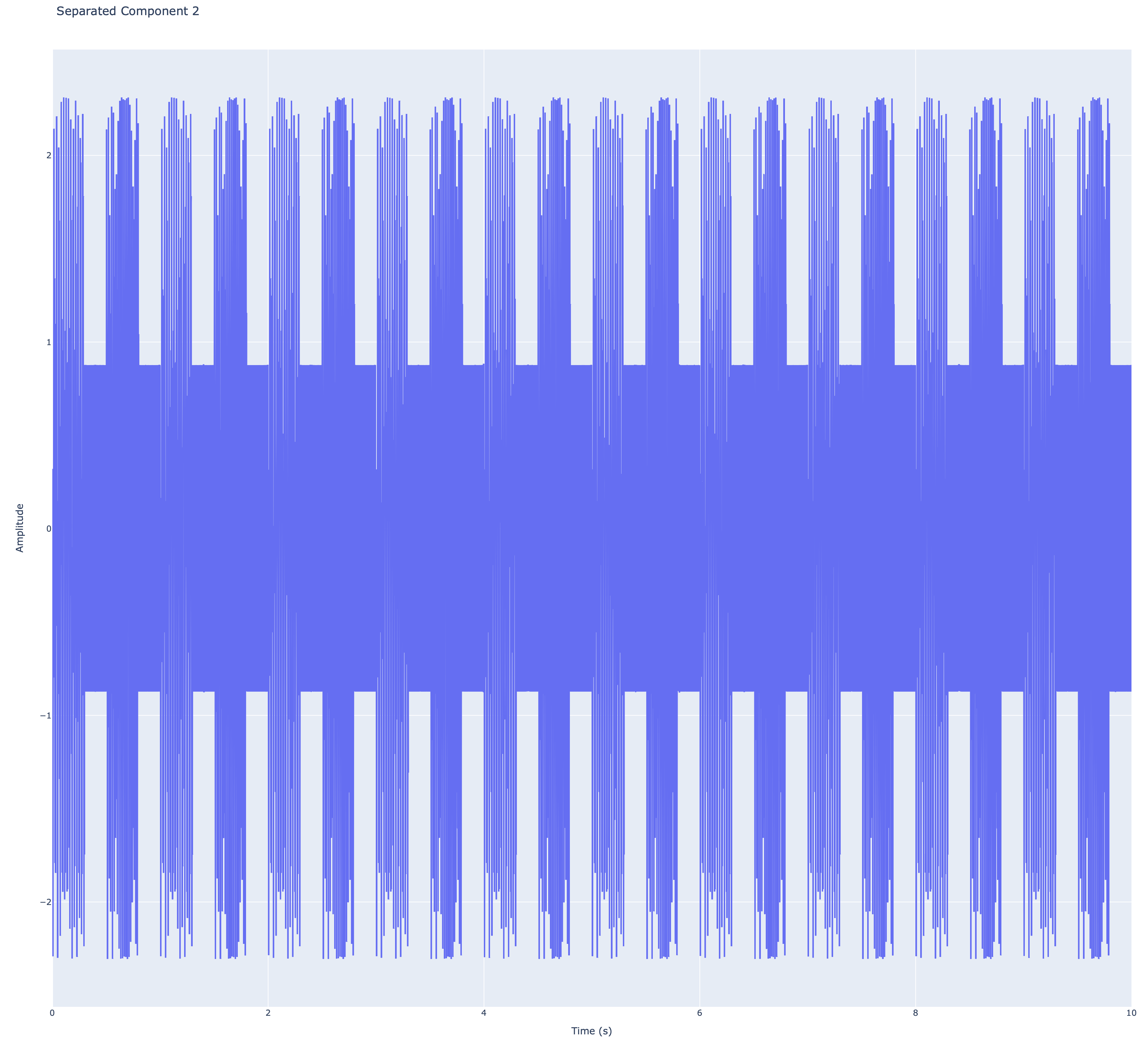
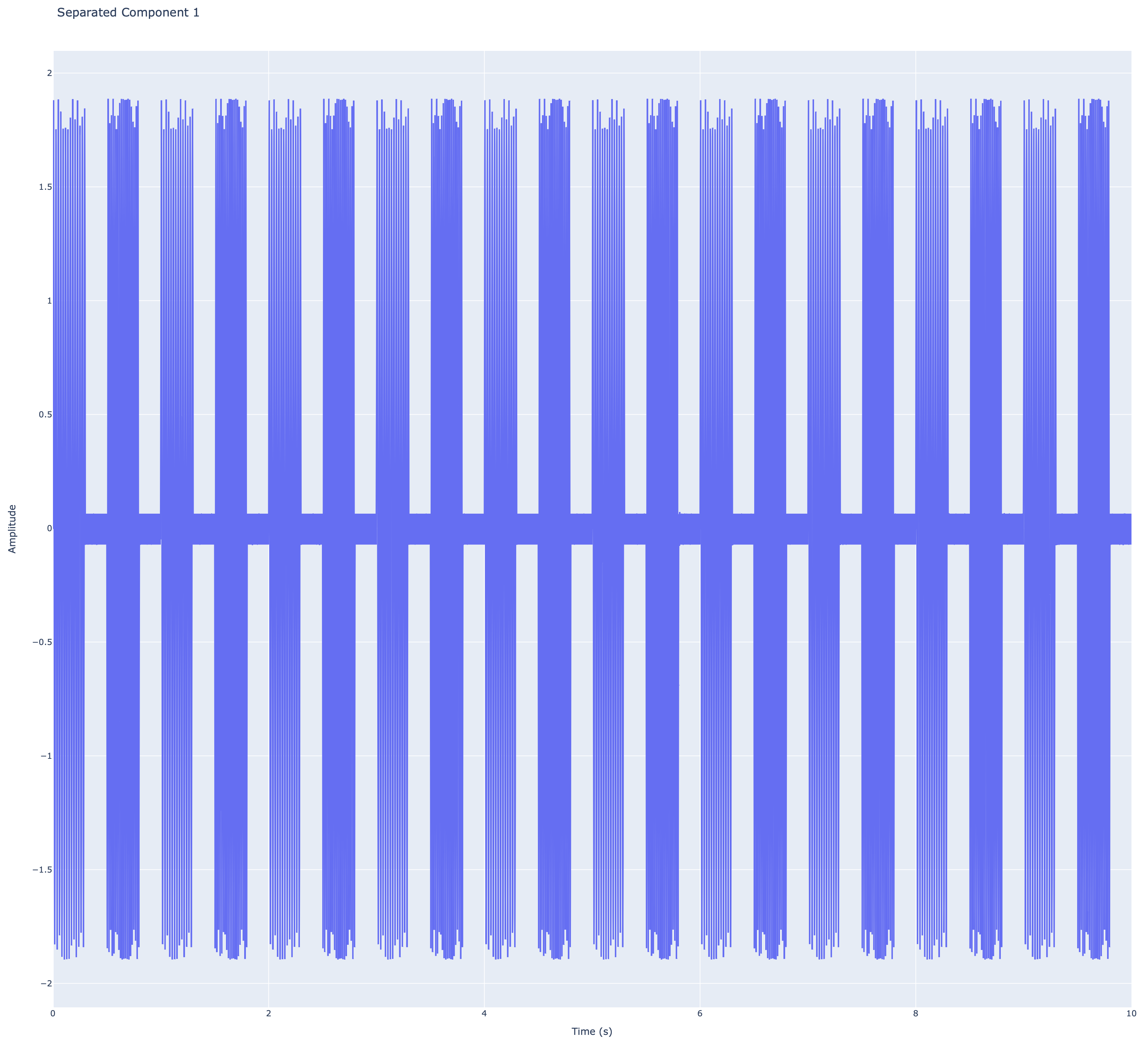
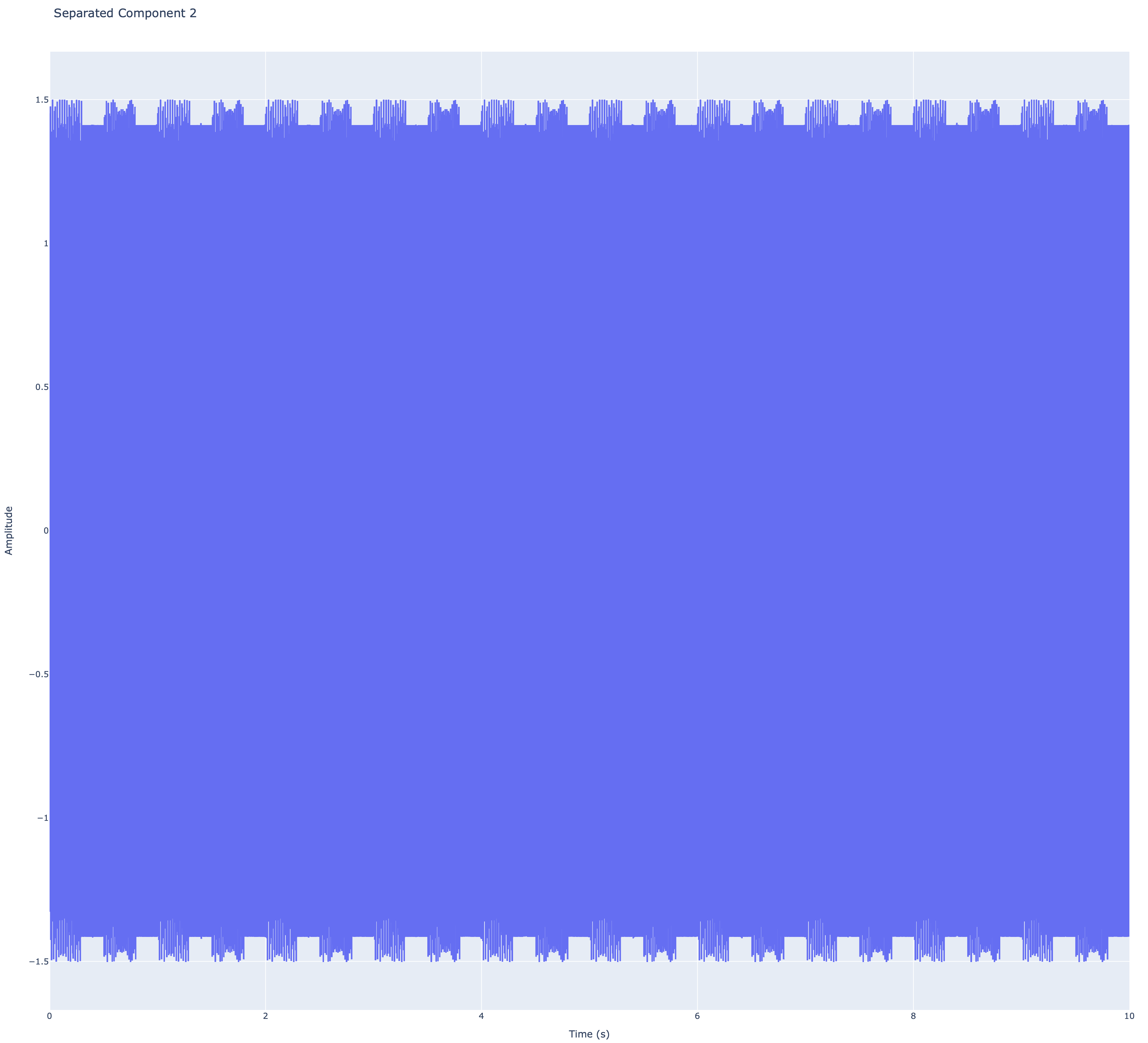
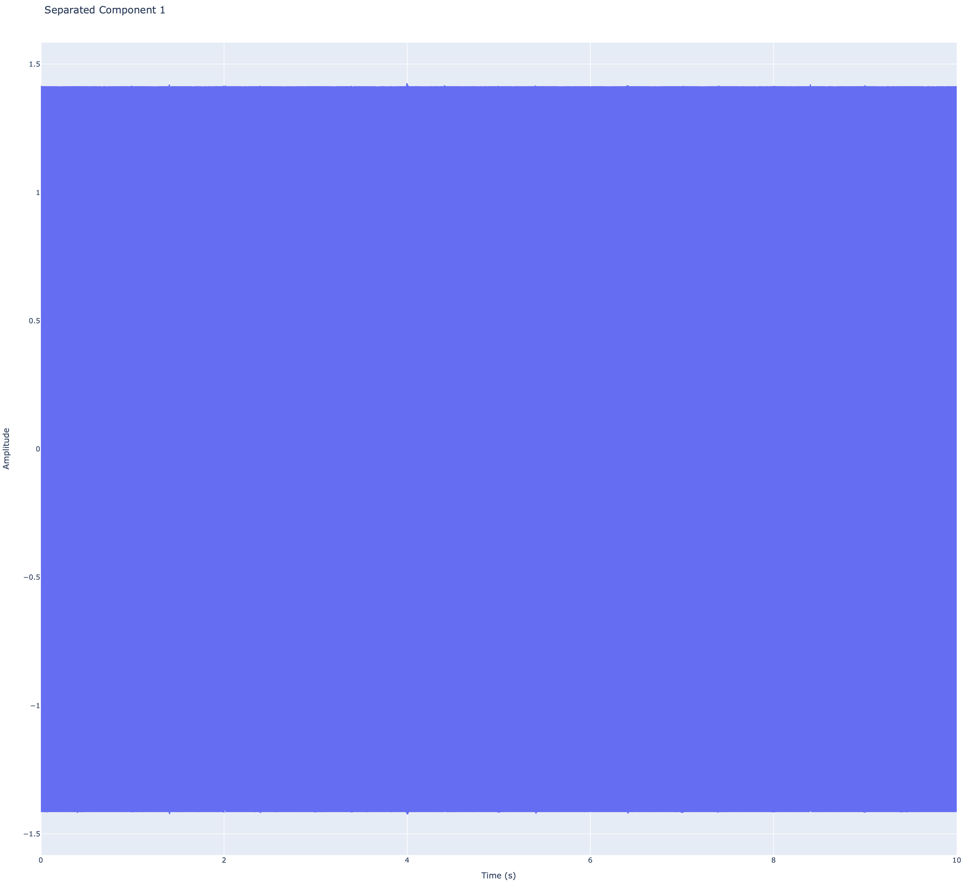
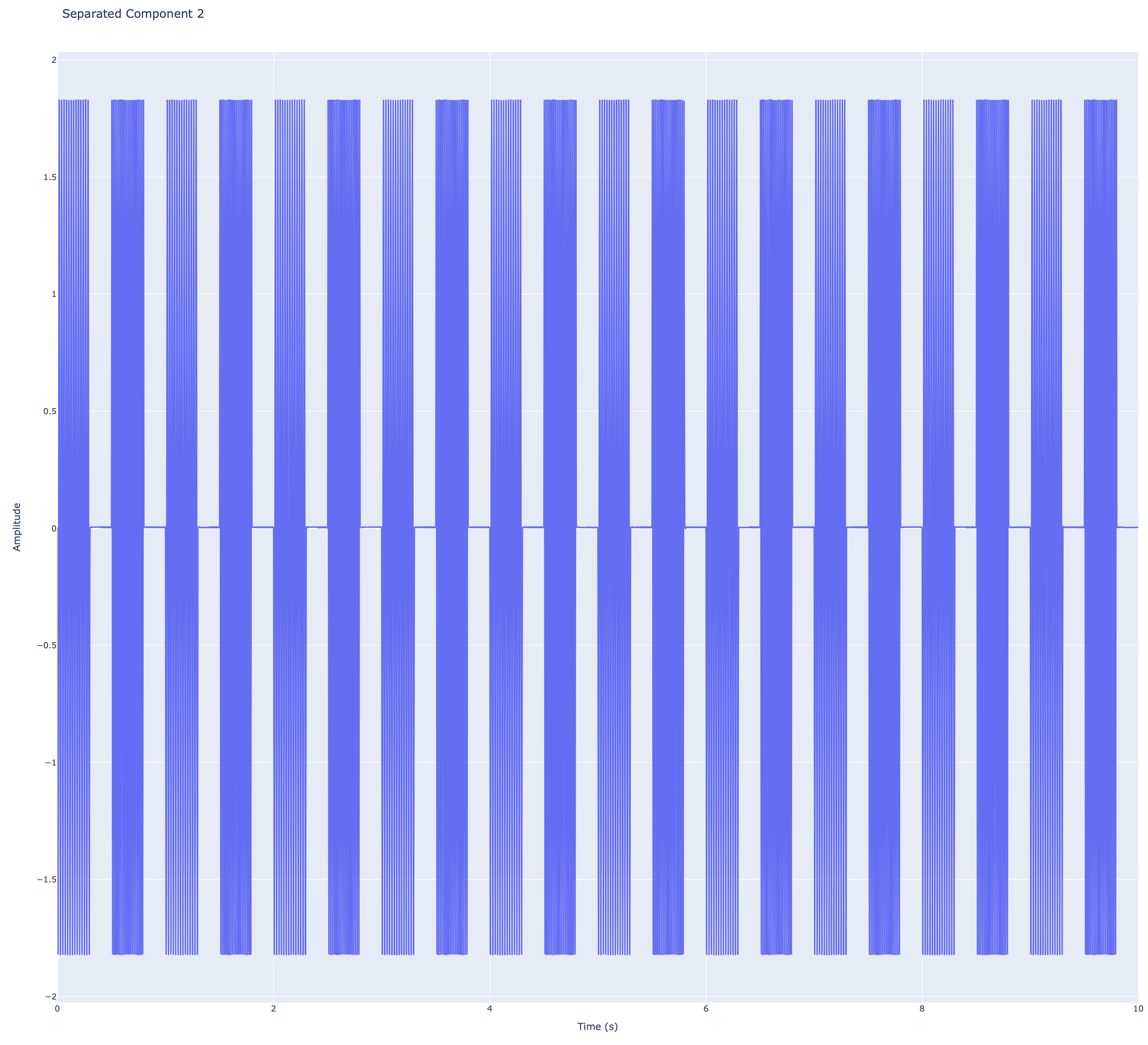
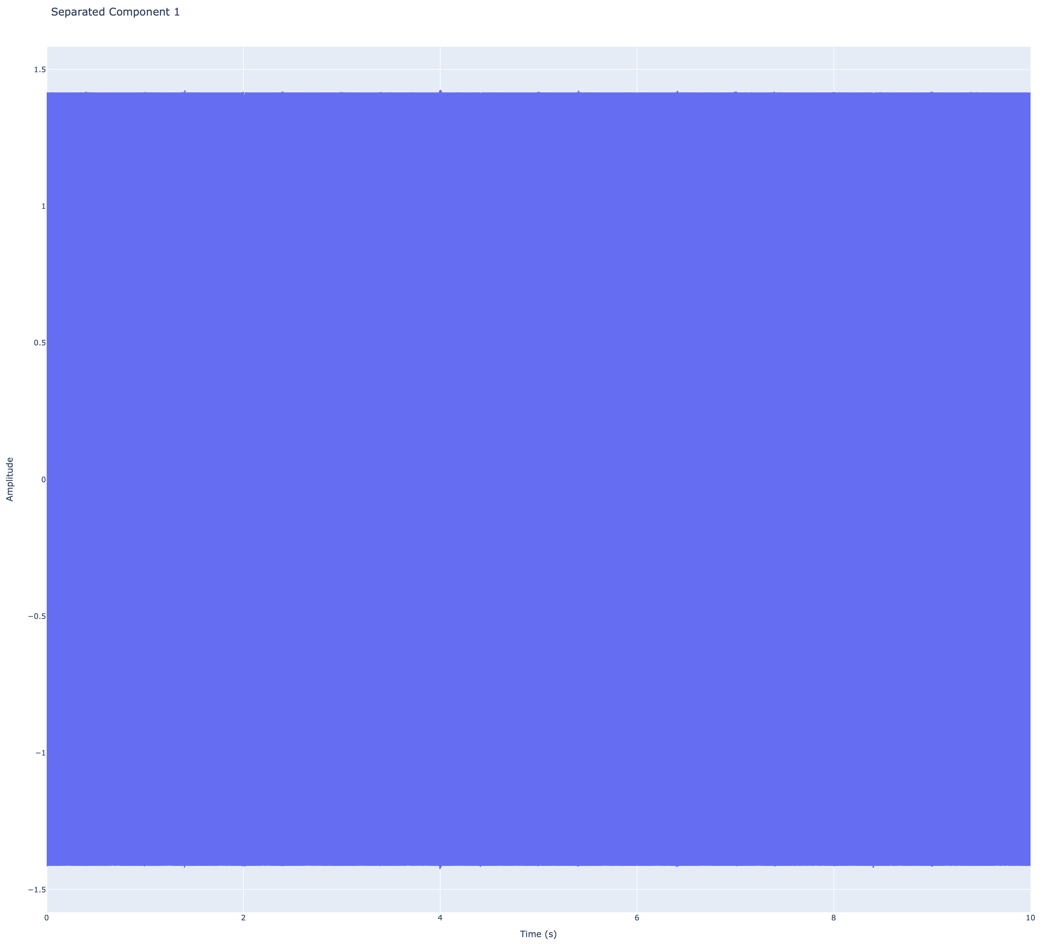
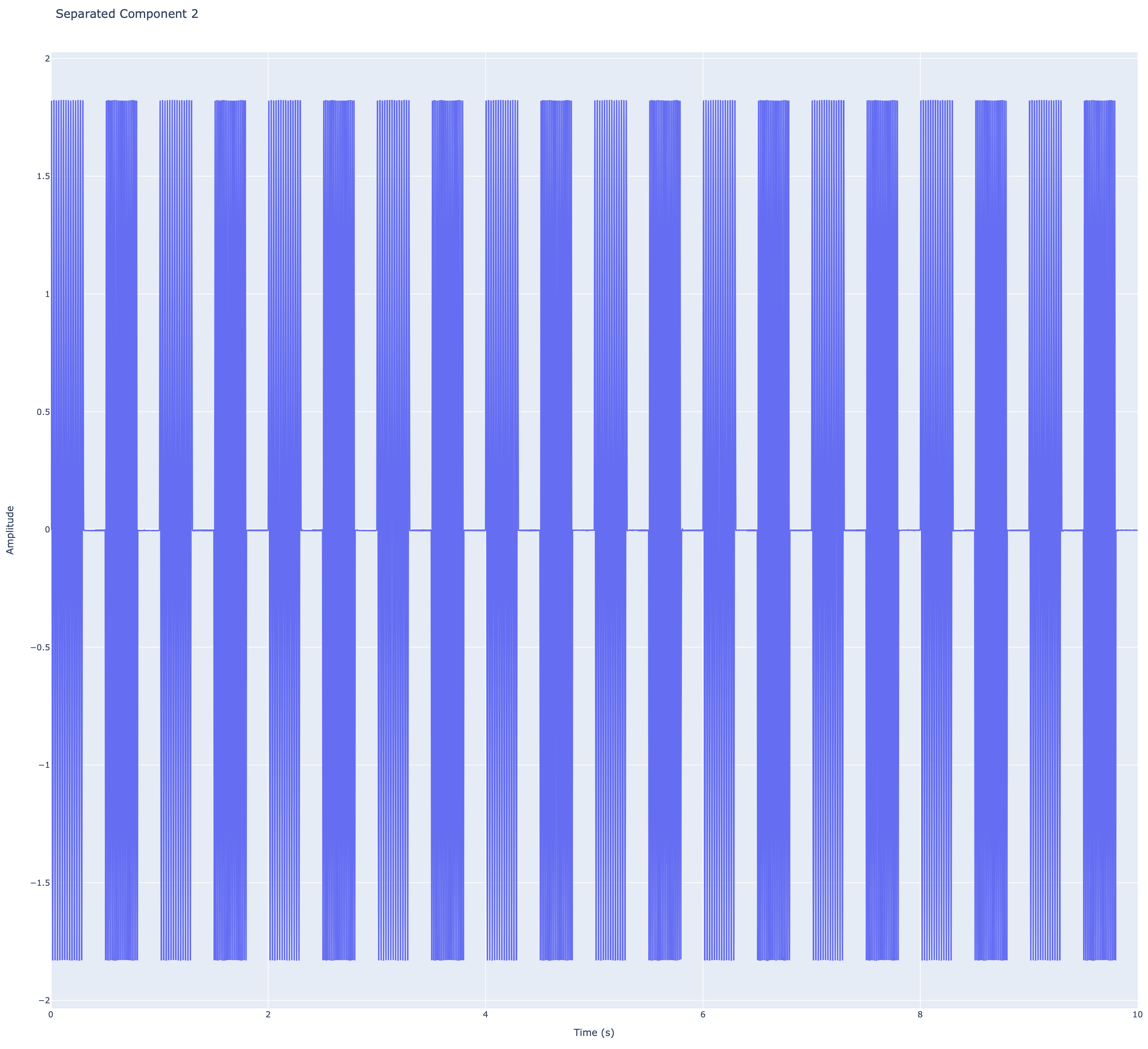
Upon executing main.py, the script generates both console output and waveform plots. These outputs demonstrate the successful integration of R scripts within Python and the effective separation of audio signals using Independent Component Analysis (ICA).
D-1) Console Output
The console output provides detailed logs of the script's execution process, including information about loading scripts, processing audio data, performing ICA, and saving the results. You can download the complete console output for further inspection:
/Users/frank/nGeneDL20241116/pythonProject/.venv/bin/python /Users/frank/nGeneDL20241116/pythonProject/main.py
Using R code from file: fastICA.R
2024-11-17 06:50:35,274 - nGene_rpy2 - INFO - Detected R installation: R version 4.4.1 (2024-06-14)
2024-11-17 06:50:35,274 - nGene_rpy2 - DEBUG - Activated numpy2ri and pandas2ri for automatic data conversion.
2024-11-17 06:50:35,274 - nGene_rpy2 - DEBUG - Initialized internal dictionaries for packages and scripts.
2024-11-17 06:50:35,276 - nGene_rpy2 - INFO - Loaded R script into package 'DefaultPackage'.
2024-11-17 06:50:35,276 - nGene_rpy2 - INFO - Loaded R script from file 'fastICA.R' into package 'DefaultPackage'.
2024-11-17 06:50:35,276 - nGene_Waveform - DEBUG - Initialized nGene_Waveform instance.
2024-11-17 06:50:35,278 - nGene_Waveform - INFO - Fetched and normalized audio data from 'heart_sound.wav'.
2024-11-17 06:50:35,278 - nGene_Waveform - INFO - Fetched and normalized audio data from 'lung_sound.wav'.
2024-11-17 06:50:35,279 - nGene_rpy2 - DEBUG - Retrieved fastICA package successfully.
2024-11-17 06:50:35,281 - nGene_rpy2 - DEBUG - Converted NumPy array to R matrix.
2024-11-17 06:50:35,281 - nGene_rpy2 - DEBUG - Retrieved R function 'fastICA' from package.
2024-11-17 06:50:35,319 - nGene_rpy2 - INFO - Called R function 'fastICA' successfully.
2024-11-17 06:50:35,319 - nGene_rpy2 - INFO - Executed fastICA function successfully.
2024-11-17 06:51:13,560 - nGene_Waveform - INFO - Plotted waveforms successfully.
2024-11-17 06:51:13,562 - nGene_Waveform - INFO - Saved separated signal 1 to 'separated_signal_1.wav'.
2024-11-17 06:51:13,564 - nGene_Waveform - INFO - Saved separated signal 2 to 'separated_signal_2.wav'.
D-2) Waveform Plot
The waveform plot visualizes the original, mixed, and separated audio signals, providing a clear representation of the ICA process. You can view the waveform plot below or download the image for your records:
nGene Waveform Studio (javascript), for Independent Component Analysis (ICA)
Guide to nGene Waveform Studio v 3.3.5
Topic
Details
Purpose
Two-column HTML5 studio for audio/video playback, live signal visualization, lightweight tempo analysis, and simple source–mixture experiments.
Pure vanilla JS; SVG-only waveforms; no frameworks or Canvas. New in v 3.3.5 line (3.3.1–3.3.5):Trim (loop-based clip creation with auto-download), matrix-based Mix of the last two items, and ICA separation of stereo mixes into two mono sources.
Layout
Left column: Player (seek/loop, playhead cursor, volume, speed, transport controls, playlist, uploads).
Right column: Trim · Mix · ICA toolbar, Tempo details panel, and Signal views (Overview, Mid, Micro, and band rows: Low/Mid/High).
File locations
Place nws.html anywhere.
Primary playlist: ./playlist.json (same folder as nws.html).
Legacy/fallback playlist and tempo meta: optional sibling folder /media/ containing playlist.json and tempo_meta.json.
Files should be world-readable (e.g., chmod 644 *).
Playlist
On load, the player first attempts ./playlist.json (array of media entries, order preserved); if unavailable, a legacy /media/playlist.json is attempted.
Absent JSON → starts empty and awaits uploads (drag-&-drop or picker).
Uploaded files are referenced via blob-URLs only (no disk writes).
Playlist ordering
Each row contains a dedicated ↓ button that sends that item directly to the bottom of the playlist while preserving the order of all others.
The currently selected row remains highlighted; index bookkeeping is adjusted so that the audible selection is preserved when possible.
Trim
Trim cuts the current loop range of the selected item into a new media item and appends it to the playlist, then immediately plays it.
Audio items: decoded into an AudioBuffer, sliced in the loop interval, given short fade-in/fade-out ramps, encoded as 16-bit PCM WAV, and added as a new playlist entry.
Video items: preferred path uses MediaRecorder on a captureStream() of the element over the loop range, targeting MP4 when supported and falling back to WebM; a pure audio WAV fallback is used when capturing A/V is not possible.
New in v 3.3.4–3.3.5: the trimmed clip is auto-downloaded using the same filename shown in the playlist (WAV or MP4/WebM), immediately after creation.
Mix (matrix A)
Mix combines the last two playlist entries into a stereo mixture using a fixed 2×2 mixing matrix: A = [[1, 1], [0.5, 2]], where rows index output channels (L,R) and columns index sources (S1,S2).
Processing: each source is downmixed to mono, linearly resampled to a common sample rate, then mixed by A with automatic peak-based scaling to avoid clipping.
Output: stereo WAV blob (L = mixture#1, R = mixture#2), auto-named as MixA_S1+S2_YYYYMMDDhhmmss.wav, appended to the playlist, and auto-selected for playback. Tempo metadata and overview are computed for the mix and stored under its filename.
ICA separation
ICA operates on the currently selected stereo item (e.g., a Mix result).
Internals: 2×N mixtures are centered, whitened via a 2×2 symmetric eigendecomposition, then separated with a 2-component FastICA (tanh nonlinearity, symmetric decorrelation between components, Frobenius-norm convergence).
Output: two mono WAV signals (ICA_A_of_* and ICA_B_of_*), normalized with modest headroom and short fades, appended to the playlist as independent entries with their own tempo and overview metadata.
Decoding & fallback
Primary decoding path: decodeAudioData on fetched/uploaded bytes. For playlist URLs, fetch is attempted first.
Fallback: full-length or range-limited capture via MediaElementSource → AudioWorklet (preferred) or ScriptProcessor, routed through a zero-gain node to keep the capture path inaudible. The muted property is never used in logic.
Tempo metadata
If present, /media/tempo_meta.json (keyed by filename) provides BPM and auxiliary fields (confidence, beat period, half/double suggestions, textual tempo class), which are reflected both in the playlist badge and the Tempo details panel.
Otherwise, an internal estimator runs on decoded buffers or short capture segments, yielding approximate BPM and beat-period values sufficient for exploratory work.
Uploads
Accessible uploader with ➕ Upload button and drag-&-drop support; the uploader itself is keyboard-focusable.
Typical formats: MP3, M4A, FLAC, WAV, OGG, AAC, and common video containers such as MP4, MOV, WebM, MKV, and AVI.
First-30-second cue
Uploader border and hint text gently pulse every 2 s for the first 30 s after load, encouraging an initial user gesture that reliably resumes the AudioContext on modern browsers.
A–B Looping
Seek bar shows cerulean A (“[”) and B (“]”) handles plus a thin ultramarine loop fill, always constrained within the gray full-track bar.
✖ Clear restores full-length playback. During playback, when the playhead reaches B, it wraps to A (with a small tolerance) as long as the loop is active.
Playhead
Current time is indicated by a vertical “I”; the center of that stroke corresponds to the true position. The playhead is draggable and is clamped within the current loop range.
Click-to-toggle video
Single-click on the video element toggles play/pause; double-click toggles fullscreen. The central ⏸︎/▶︎ transport button remains synchronized with element state.
Autoplay
The first playlist item may start automatically depending on browser autoplay policy. The AudioContext resumes on the first user interaction (click, drag, drop, or keyboard action) to ensure consistent audio routing.
Repeat Mode
Repeat cycles between One (🔁 with “1”), All (🔁), and Off (⛔).
With an A–B loop active, playback wraps within the loop regardless of repeat mode. When the loop is cleared, Repeat = All advances across playlist items; Repeat = One replays the same item.
Smooth range input with live “elapsed / total” time label, draggable A–B handles, thin loop fill, and a precise “I”-shaped cursor.
Loop bounds constrain both seeking and continuous playback; a small, duration-dependent epsilon avoids stickiness at the upper boundary during wrap.
Volume
0–500 % via WebAudio GainNode (primary route, single audible path).
If WebAudio is unavailable, a graceful fallback uses native element volume (0–100 %). The design avoids double-routing and unintended parallel audio paths.
Speed
0.05× – 2.00× with − / + step buttons (0.01 increments) and a 1× reset button. The same playback rate is applied to both audio and video media elements.
Tempo details
Tempo panel presents BPM (with confidence), beat period (ms), half/double candidates, tempo class (Slow/Moderate/Fast), and effective BPM at the current playback speed (BPM × rate).
The panel is visible whenever either file-based metadata or the internal estimator provides data for the selected item.
Overview (playlist.json-aware)
Overview is a whole-file SVG representation built from min/max envelopes over fixed buckets. In v 3.3.5, an internal helper ensures that an Overview is generated for the currently selected item even when it comes from playlist.json loaded at startup (audio or video).
Once constructed, the same Overview supports both the main Overview view and the centered Micro view around the playhead.
Signal views
Overview (entire file, absolute timebase, interactive loop brackets and cursor), Mid (live trailing window, default 8 s), and Micro (centered ±3 s around the playhead; falls back to trailing when no Overview is available).
Band rows (Low ≤~200 Hz, Mid ~200–2000 Hz, High ≥~2 kHz) use a simple one-pole filter bank per band and share the same trailing length as the Mid window, with distinct color-coded strokes for quick visual discrimination.
Live tap
AudioWorklet-based collector (preferred) or ScriptProcessor fallback receives data from the shared MediaElementSource nodes via an inaudible zero-gain branch.
Envelope rings are filled at an effective rate of ~2 kHz and decimated to maintain responsiveness while limiting CPU load. Tap operations do not alter the audible signal.
Resizable wrapper
Outer .wrapper uses resize:both; the default width is governed by --w (980 px), suitable for dual-column layouts on desktop screens.
The playlist panel is vertically resizable, allowing adaptation to longer track lists or small windows.
Accent colour
Changing --accent (default #1e90ff) rebrands key UI elements, including buttons, sliders, pulse highlights, and active playlist rows, while preserving structural CSS.
Fullscreen
The ⛶ button and the F key toggle fullscreen for video items only; audio items retain the compact layout. The output route is re-applied on fullscreen changes to maintain consistent gain behaviour.
Source-code reveal
Embedded “Full Source Code” accordion shows the entire page’s HTML/JS/CSS, syntax-highlighted via Highlight.js, allowing inspection, copy-paste, and regression testing from a single file.
Namespace
All logic resides inside a single IIFE; public surface is limited to instantiation of the WaveformStudio class against the #box container. CSS is scoped by class names to minimize interaction with surrounding pages or frameworks.
Notes & caveats
Decoding and cross-origin fetching depend on server CORS configuration; when direct decoding fails, the capture-based fallback is used instead. Some exotic codecs or DRM-protected streams may remain unsupported.
Mixed, trimmed, and ICA-derived outputs are held as in-memory blobs and appear as playlist entries; only Trim explicitly triggers a download by default in v 3.3.5.
Guide to nGene Waveform Studio v 3.1.0
Topic
Details
Purpose
Two-column HTML5 studio for audio/video playback, live signal visualization, and lightweight tempo analysis.
Pure vanilla JS; SVG-only waveforms; no frameworks or Canvas. New in v 3.1.0:Mix button (right column) that combines the last two playlist items into a headroom-safe WAV and appends it to the playlist for immediate playback.
Layout
Left column: Player (seek/loop, volume, speed, transport, playlist, uploads).
Right column: Mix toolbar, Tempo details panel, and Signal views (Overview, Mid, Micro, and band rows).
File locations
Place nws.html anywhere.
Optional sibling folder /media/ for playlist.json and tempo_meta.json.
Ensure readable permissions (e.g., chmod 644 *).
Playlist
Optional /media/playlist.json — array of media paths (order preserved).
Absent JSON → starts empty and awaits uploads (drag-&-drop or picker).
Uploaded files are referenced via blob-URLs (no disk writes).
Mix (new)
Click Mix to combine the last two playlist entries (audio or the audio track of video).
Processing: OfflineAudioContext offline render; per-track gain = 0.5 for headroom; linear sum; length = max(duration).
Output: in-memory WAV blob, auto-named as Mix - A + B.wav, appended to the playlist, and auto-played. Status text reports progress or errors (e.g., CORS/decoding).
Decoding & fallback
Primary: decodeAudioData on fetched/uploaded bytes.
Fallback: full-length capture via MediaElementSource → Worklet/ScriptProcessor (kept inaudible through a zero-gain node; no muted property used).
Tempo metadata
If available, /media/tempo_meta.json (keyed by filename) populates BPM and related fields in the list and Tempo panel.
When absent, a quick internal estimator computes approximate BPM/beat period from short decoded segments or short captures.
Uploads
➕ Upload button and drag-&-drop; keyboard focusable uploader.
Uploaded audio/video formats commonly supported: MP3/M4A/FLAC/WAV and MP4/MOV/WEBM/MKV/AVI.
First-30-second cue
Uploader border and hint gently pulse every 2 s for the first 30 s after load to encourage interaction (resumes AudioContext reliably).
A–B Looping
Seek bar shows cerulean A (“[”) and B (“]”) handles and a thin ultramarine loop fill, always inside the gray full-track bar.
✖ Clear restores full-length playback instantly.
Playhead
Current time indicated by a vertical “I”; the center of the line is the true position. Draggable, clamped within the loop.
Click-to-toggle video
Single-click on video toggles play/pause; double-click toggles fullscreen. The ⏸︎/▶︎ control remains synchronized.
Autoplay
First item may start automatically (per browser policy). AudioContext resumes on first user gesture (click, drag, drop) for consistent sound.
Repeat Mode
Cycles: One (🔁 with “1”) → All (🔁) → Off (⛔).
With a loop active, playback wraps to loop start. After clearing loop and with Repeat = All, playback advances to the next track.
Smooth range input with live “elapsed / total”, draggable A–B handles, thin loop fill, and precise “I” cursor.
Loop bounds clamp seeking and playback, with edge-aware wrap to loop start.
Volume
0–500 % via WebAudio GainNode (primary route).
Graceful fallback uses element volume (0–100 %) if WebAudio is unavailable. Single audible route is always maintained.
Speed
0.05× – 2.00× with − / + step buttons (0.01) and 1× reset. Applies to audio and video uniformly.
Tempo details
BPM (with confidence), beat period (ms), half/double suggestions, tempo class (Slow/Moderate/Fast), and effective BPM at current speed.
Panel appears when data are available (from metadata file or internal estimator).
Signal views
Overview (whole file; absolute “now” marker), Mid (live trailing window, default 8 s), Micro (centered ±3 s around playhead;
falls back to trailing if overview not ready), and Band rows (Low ≤~200 Hz, Mid ~200–2000 Hz, High ≥~2 kHz) with color-coded strokes.
Window lengths selectable; ✖ clears live buffers.
Live tap
AudioWorklet collector (preferred) or ScriptProcessor fallback feeds envelope rings at ~2 kHz sampling for responsive SVG paths.
Capture remains inaudible through a zero-gain branch; no reliance on muted.
Resizable wrapper
Outer .wrapper uses resize:both; default width from --w (980 px for two columns).
Track list is vertically resizable.
Accent colour
Adjust --accent (default #1e90ff) to rebrand buttons, sliders, uploader, and active highlights.
Fullscreen
Dedicated ⛶ button and keyboard F toggle fullscreen for video items.
Source-code reveal
Built-in “Full Source Code” accordion displays the whole page, syntax-highlighted via Highlight.js, for sharing and tests.
Namespace
All logic is encapsulated in an IIFE; CSS classes are locally scoped. Safe to embed alongside other pages and scripts.
Notes & caveats
Decoding and cross-origin fetching depend on server CORS policies; when decoding fails, the inaudible capture fallback is attempted.
Mixed output is stored as an in-memory blob (download prompt is not issued automatically).
Guide to nGene Media Player v 2.6
Topic
Details
Purpose
Self-contained, resizable HTML5 media player for audio
(MP3/M4A/FLAC/WAV) and video (MP4/MOV/WEBM/MKV/AVI).
Pure vanilla JS—no frameworks. New since v 2.6: vertical “I” playhead
(center = true position), refined A–B loop visuals, hardened uploads/drag-&-drop,
reliable play/pause with AudioContext resume.
File locations
Place nmp.html anywhere.
Media files live in sibling /media/.
Ensure readable permissions, e.g., chmod 644 *.
Playlist
Optional /media/playlist.json — array of media paths (order preserved).
If absent, player starts empty and waits for user uploads.
Tempo metadata
Player reads tempo_meta.json (keyed by filename)
to show integer-rounded BPM beside each track
and in the title line (e.g., “128 BPM”).
Uploads
➕ Upload button and drag-&-drop.
Files are played via blob-URLs (no disk writes).
The dashed uploader box is clickable and keyboard-focusable.
First-30-second attention cue
Uploader border and hint softly pulse/glow every 2 s
for the first 30 s after load.
A–B Looping
Seek bar shows two cerulean brackets:
• A handle “[” — loop start.
• B handle “]” — loop end.
Ultramarine blue loop bar (thinner) fills the loop region
and is always fully inside the gray full-length bar (entire track).
✖ Clear resets loop to full-length instantly.
Playhead
Current position is a vertical “I” line;
its center is the true time point.
It can be dragged, and is always clamped inside the blue loop bar.
Click-to-toggle video
Click anywhere on the visible video to play/pause;
⏸︎/▶︎ stays in sync. Double-click toggles fullscreen.
Autoplay
First item starts automatically (subject to browser policy).
AudioContext is resumed on first user gesture
(e.g., button, drag, drop) for reliable playback.
Repeat Mode
Cycles: 🔂 One → 🔁 All → ⛔ Off.
With a loop active, playback wraps to the loop start.
After you press ✖ to clear loop and Repeat = All,
the player advances to the next track at end
(not the same track).
Sleek seek bar with live “elapsed / total” timer,
A–B handles, thin blue loop bar, and draggable “I” playhead.
Volume
0–200 % gain via WebAudio (gain node). Default is 33 %.
If WebAudio is unavailable, falls back to element volume (0–100 %).
Speed
0.05× – 2.00× slider with − / + step buttons (0.01)
and 1× reset. Applies to both audio and video.
Resizable wrapper
Outer .wrapper uses resize:both;
default width from --w (360 px).
Track-list is vertically resizable.
Accent colour
Edit --accent (default #1e90ff)
to rebrand buttons, slider thumbs, uploader, and active track highlight.
Fullscreen
Dedicated ⛶ button and keyboard F toggle fullscreen for video items.
Source-code reveal
Built-in “Full Source Code” accordion shows the entire page,
syntax-highlighted via Highlight.js (for easy sharing/tests).
Namespace
All logic wrapped in an IIFE; CSS uses scoped class names.
Safe to embed alongside other scripts and styles.
Guide to nGene Media Player v 2.4
Topic
Details
Purpose
Self-contained, resizable HTML5 player for audio (MP3/M4A) and video (MP4/MOV/WEBM). Pure vanilla JS—no frameworks required. New since v 1.8: tempo-aware track-list showing BPM (integer-rounded), auto-loading from tempo_meta.json; initial volume defaults to 17 % at page-load.
File locations
Place nmp.html anywhere.
Media files live in a sibling /media/ folder.
Ensure readable permissions with chmod 644 *.
Playlist
Optional /media/playlist.json—an array of paths (order preserved). If absent, the player simply waits for user uploads.
Tempo metadata
Run extract_meta_from_media.py v 2.4 to generate tempo_meta.json (single integer-rounded bpm). Player displays it beside each track and in the title-bar as “### BPM”.
Uploads
➕ Upload button and drag-&-drop. Files become blob-URLs, so nothing is written to disk.
First-30-second attention cue
Uploader border, hint-text and container gently pulse, glow and scale every 2 s for the first 30 s after page-load.
A-B Looping
Seek-bar sports two cerulean “brackets”:
• A handle “[” — left edge marks loop-start.
• B handle “]” — right edge marks loop-end.
Drag to set; ultramarine bar fills the loop range. ✖ Clear button instantly resets the loop.
Click-to-toggle video
Click anywhere on the visible video to play/pause; the ⏸︎/▶︎ button stays synchronised.
Autoplay
The first track auto-starts; subsequent behaviour follows Repeat Mode.
Repeat Mode
Begins at 🔂 One (loop current). Button cycles: 🔂 One → 🔁 All → 🔁 Off.
Controls
⏮︎ Prev • ⏸︎/▶︎ Toggle • ⏭︎ Next • Repeat — plus ✖ Loop-Clear beside the seek-bar.
Seek & Time
Sleek seek-bar with live “elapsed / total” timer, integrated A-B loop handles and ultramarine fill.
Volume
Smooth 0–100 % slider with live percentage label; initial default 17 % (0.17).
Speed
0.70× – 2.00× slider with − / + step buttons and 1× reset. Applies to audio & video.
Resizable wrapper
Outer .wrapper uses resize:both; default width governed by --w (360 px). Track-list is vertically resizable.
Accent colour
Edit --accent (default #1e90ff) to rebrand buttons, slider thumbs, active-track row and uploader pulse.
Source-code reveal
Built-in “Full Source Code” accordion shows the entire page, syntax-highlighted via Highlight.js.
Namespace
All logic wrapped in an IIFE; CSS uses local class names—safe to embed anywhere.
Guide to nGene Media Player v 1.8 (c)
Topic
Details
Purpose
Self‑contained, resizable HTML5 player for audio (MP3/M4A) and video (MP4/MOV/WEBM). Pure vanilla JS—no frameworks. New since v 1.6 (c): draggable cerulean‑blue “bracket” handles for precise A‑B looping, ultramarine loop‑fill, and click‑to‑toggle playback directly on the video surface.
File locations
Place nmp.html anywhere.
Media files live in a sibling /media/ folder.
Ensure readable permissions with chmod 644 *.
Playlist
Optional /media/playlist.json—an array of paths (order preserved). If absent, the player simply waits for user uploads.
Uploads
➕ Upload button and drag‑&‑drop. Files become blob‑URLs, so nothing is written to disk.
First‑30‑second attention cue
Uploader border, hint‑text and container gently pulse, glow and scale every 2 s for the first 30 s after page‑load.
A‑B Looping (1.8 series)
Seek‑bar sports two cerulean “brackets”:
• A handle “[” — left edge marks loop‑start.
• B handle “]” — right edge marks loop‑end.
Drag to set; ultramarine bar fills the loop range. ✖ Clear button instantly resets the loop.
Click‑to‑toggle video
Click anywhere on the visible video to play/pause; the ⏸︎/▶︎ button stays synchronised.
Autoplay
The first track auto‑starts; subsequent behaviour follows Repeat Mode.
Repeat Mode (default)
Begins at 🔂 One (loop current). Button cycles: 🔂 One → 🔁 All → 🔁 Off.
Controls
⏮︎ Prev • ⏸︎/▶︎ Toggle • ⏭︎ Next • Repeat — plus ✖ Loop‑Clear beside the seek‑bar.
Seek & Time
Sleek seek‑bar with live “elapsed / total” timer. Integrates A‑B loop handles and ultramarine fill described above.
Volume
Smooth 0–100 % slider with live percentage label.
Resizable wrapper
Outer .wrapper uses resize:both; default width governed by --w (360 px). Track‑list is vertically resizable.
Accent colour
Edit --accent (default #1e90ff) to rebrand buttons, slider thumbs, active‑track row and uploader pulse.
Source‑code reveal
Built‑in “Full Source Code” accordion shows the entire page, syntax‑highlighted via Highlight.js.
Namespace
All logic wrapped in an IIFE; CSS uses local class names—safe to embed anywhere.
Waveform Analysis of Sound by Mikio Tohyama
Chapter 2: Transforms, poles, zeros, and waveform structure (Written June 5, 2026)
A sound waveform is a change in air pressure, voltage, or digital amplitude over time.
At first glance, a waveform looks like a curve on the time axis.
However, many important properties of sound are difficult to understand from the time-domain curve alone.
It is not always obvious why a sound rings for a long time, why a certain frequency is emphasized,
why a feedback system becomes unstable, or how much delay exists between two similar waveforms.
The concepts in Chapter 2 can therefore be understood as different ways of reading the same waveform.
Z-transform, Fourier transform, convolution, cross-correlation, poles, zeros, convergence, and inverse transforms
are not isolated formulas. They are tools for seeing hidden structure inside waveform behavior.
Fourier transform explains a waveform by asking, “What frequencies are inside it?” Z-transform explains a waveform system by asking, “Why does it decay, ring, resonate, or become unstable?”
I. From waveform to discrete sequence
Meaning of a discrete sequence
A physical sound signal changes continuously over time. In continuous-time notation, it can be written as:
\[
x(t)
\]
A computer cannot directly store every value of a continuous signal.
Instead, the signal is sampled at regular time intervals.
The resulting list of numbers is called a discrete sequence.
\[
x[0],\ x[1],\ x[2],\ x[3],\cdots
\]
For example, a 44.1 kHz audio signal contains 44,100 samples per second.
Each sample represents the amplitude of the waveform at a specific time.
\[
x[n]
\]
In digital sound analysis, the waveform is therefore represented as a discrete sequence.
When drawn as a graph, it appears as a waveform. When written mathematically, it appears as a sequence.
Illustration: A digital waveform is a sequence of sampled amplitudes.
When these values are placed in time order, they form a waveform.
Thus, a discrete sequence is not a separate abstraction detached from sound.
In digital audio, it is the basic representation of the waveform itself.
All later operations start from this sequence \(x[n]\).
Z-transform, Fourier transform, convolution, and cross-correlation are all methods for analyzing or manipulating this sequence.
II. Convolution: applying a system to a waveform
Meaning of convolution
Convolution is the operation that calculates the output waveform produced when an input waveform passes through a system.
It is written as:
\[
y[n]=x[n]*h[n]
\]
In expanded form:
\[
y[n]=\sum_{k=-\infty}^{\infty}x[k]h[n-k]
\]
Here, \(x[n]\) is the input waveform, \(h[n]\) is the system impulse response,
and \(y[n]\) is the output waveform.
Meaning of impulse response
An impulse response describes how a system reacts to a very short input.
A simple acoustic example is a hand clap in a room.
The clap itself is brief, but the room continues to respond through reflections and reverberation.
The room response to that short clap is the impulse response.
When another sound passes through the same room, the resulting reverberant sound can be understood as the convolution
of the original sound with the room impulse response.
Illustration: A short impulse becomes a decaying reverberation tail after convolution with a system response.
Reason for using convolution
Many acoustic and audio systems can be described by the combination of an input waveform and a system response.
Convolution is used to calculate this combination.
Typical examples include:
Room reverberation
Echo
Loudspeaker response
Microphone coloration
Digital filters
Headphone or earphone acoustic response
In this sense, convolution explains how a waveform changes after passing through an environment, device, or filter.
III. Cross-correlation: finding similarity and delay between waveforms
Meaning of cross-correlation
Cross-correlation measures the similarity between two waveforms.
More specifically, one waveform is shifted along the time axis, and the operation checks at which shift the two waveforms match best.
A common form is:
\[
R_{xy}[m]=\sum_n x[n]y[n+m]
\]
Here, \(m\) is the time lag.
If \(R_{xy}[m]\) becomes large at a certain \(m\), the two waveforms are most similar at that delay.
Illustration: The peak of cross-correlation indicates the delay where two waveforms align best.
Reason for using cross-correlation
In acoustics, it is often important to find the time difference between related signals.
For example, an original sound and its reflected echo may have similar shapes but different arrival times.
Cross-correlation can reveal that time delay.
Cross-correlation is used for:
Echo delay estimation
Pitch detection
Room impulse response measurement
Time delay estimation in microphone arrays
Sound source localization
Difference between convolution and cross-correlation
Convolution creates an output waveform by applying a system response to an input waveform.
Cross-correlation compares two waveforms and finds the delay at which they are most similar.
Concept
Main question
Acoustic meaning
Convolution
What waveform is produced after this system?
Reverb, echo, filtering
Cross-correlation
At what delay do two waveforms match best?
Delay, pitch, echo position
IV. Z-transform: a language for reading waveform systems
Definition of Z-transform
The Z-transform converts a discrete sequence \(x[n]\) into a function \(X(z)\) of a complex variable \(z\).
\[
X(z)=\sum_{n=-\infty}^{\infty}x[n]z^{-n}
\]
The variable \(z\) is complex:
\[
z=re^{j\omega}
\]
Therefore, the Z-transform changes a time-domain waveform into a function that can be analyzed on the complex plane.
Real reason for using Z-transform
The purpose of the Z-transform is not merely to make formulas shorter.
Its deeper purpose is to reveal the overall behavior of a waveform system without following every sample one by one.
Consider the following system:
\[
y[n]=x[n]+0.8y[n-1]
\]
This means that the current output \(y[n]\) depends not only on the current input \(x[n]\),
but also on the previous output \(y[n-1]\).
In other words, 80% of the previous output remains in the current output.
This structure is related to reverberation, ringing, resonance, and feedback.
A sound does not disappear immediately; part of the previous sound remains and continues into the next sample.
Complexity in the time domain
In the time domain, the equation expands as follows:
The current output is therefore not determined only by the current input.
It contains an infinite accumulation of past inputs, each weighted by a decreasing factor.
From the time-domain equation alone, the following questions are not immediately simple:
Is the system stable?
Does the sound decay or grow over time?
Which frequencies are emphasized?
Which frequencies are weakened?
What does the impulse response tail look like?
Simplicity in the Z-domain
The Z-transform turns a delay into multiplication:
From this single expression, stability, frequency response, impulse response, and pole location can be read.
Relation between Z-transform and waveform
If an impulse is applied to the system:
\[
x[n]=\delta[n]
\]
the output becomes:
\[
h[n]=0.8^n u[n]
\]
That is:
\[
1,\ 0.8,\ 0.64,\ 0.512,\ 0.4096,\cdots
\]
This is a decaying waveform tail.
Acoustically, it resembles a sound that gradually disappears after being excited.
The Z-transform explains why this waveform has that tail.
Without calculating every sample in the time domain, \(H(z)\) reveals what kind of waveform behavior the system will produce.
Illustration: A pole inside the unit circle creates decay, while a pole outside the unit circle creates growth.
V. Convergence and inverse Z-transform
Meaning of convergence
The Z-transform is an infinite sum:
\[
X(z)=\sum_{n=-\infty}^{\infty}x[n]z^{-n}
\]
This sum does not necessarily converge for every value of \(z\).
The set of \(z\)-values for which the sum converges is called the Region of Convergence, or ROC.
Convergence tells where the expression has mathematical meaning.
It is also closely related to causality and stability.
Convergence and waveform tail
Consider:
\[
x[n]=0.8^n u[n]
\]
This sequence decreases over time:
\[
1,\ 0.8,\ 0.64,\ 0.512,\cdots
\]
Its waveform tail decays and remains stable.
By contrast:
\[
x[n]=1.2^n u[n]
\]
increases over time:
\[
1,\ 1.2,\ 1.44,\ 1.728,\cdots
\]
In this case, the waveform grows instead of disappearing.
Thus, convergence is directly related to whether a waveform is stable or divergent.
Meaning of inverse Z-transform
The inverse Z-transform converts a Z-domain expression back into a time-domain sequence.
\[
X(z)\rightarrow x[n]
\]
For example, if:
\[
X(z)=\frac{1}{1-0.8z^{-1}}
\]
and the sequence is causal, the corresponding time-domain sequence is:
\[
x[n]=0.8^n u[n]
\]
The inverse Z-transform therefore returns complex-plane analysis to an actual waveform sequence.
VI. Poles and zeros: a map of system behavior
Basic form of a transfer function
In the Z-domain, a system is often expressed as:
\[
H(z)=\frac{B(z)}{A(z)}
\]
Here, \(B(z)\) is the numerator and \(A(z)\) is the denominator.
Zeros and poles come from this expression.
Meaning of a zero
A zero is a value of \(z\) that makes the transfer function equal to zero.
\[
H(z)=0
\]
In other words:
\[
B(z)=0
\]
A zero weakens or removes a certain component.
If a zero lies on the unit circle, the frequency corresponding to that angular position can be strongly suppressed.
Acoustically, this is related to a notch filter.
For example, a zero can be placed at a frequency corresponding to a hum noise in order to reduce that component.
A zero therefore removes or weakens a particular oscillatory component inside a waveform.
Meaning of a pole
A pole is a value of \(z\) where the transfer function becomes very large.
It occurs when the denominator becomes zero:
\[
A(z)=0
\]
A pole tends to maintain or amplify a certain component.
Suppose a pole is located at:
\[
p=re^{j\omega_0}
\]
In the time domain, it produces a component similar to:
\[
r^n e^{j\omega_0 n}
\]
Here, \(r\) is related to decay speed, and \(\omega_0\) is related to oscillation frequency.
If \(r\) is close to 1, the sound decays slowly.
The waveform then has a long ringing or resonance.
Meaning of an unstable pole
In a causal discrete-time system, a pole outside the unit circle is unstable.
\[
|p|>1
\]
For example, if:
\[
p=1.2
\]
the impulse response grows as:
\[
1.2^n
\]
The waveform does not decay. Instead, it grows over time.
Acoustically, this resembles microphone-speaker feedback.
If a microphone receives the loudspeaker output, the signal is amplified and played again.
When the loop gain is too large, a certain frequency grows repeatedly and produces a strong feedback tone.
Reason for using a pole-zero plot
A pole-zero plot is a map of system behavior.
A waveform may look complicated in the time domain,
but the positions of poles and zeros reveal why the waveform rings, decays, resonates, or becomes unstable.
Illustration: The unit circle separates stable causal pole locations from unstable ones. Zeros suppress components.
Observed behavior
Pole-zero interpretation
Waveform result
Removal of a frequency
A zero is located near that frequency
The corresponding oscillation becomes weaker
Resonance
A pole is located near the unit circle
Ringing or resonance appears
Fast decay
The pole radius is small
The tail disappears quickly
Long decay
The pole is close to the unit circle
The tail remains for a long time
Instability
The pole is outside the unit circle
The waveform amplitude grows over time
VII. Fourier transform: reading a waveform as frequency content
Meaning of Fourier transform
Fourier transform interprets a waveform as a sum of sinusoidal components.
Even a complicated waveform can be analyzed as a combination of many frequencies.
In the time domain, the signal is written as:
\[
x[n]
\]
After Fourier transform, the signal is represented by its frequency content:
Illustration: A complex sound can be understood as a set of spectral peaks such as a fundamental and harmonics.
Reason for using Fourier transform
Sound may look complex on the time axis, but its structure is often clearer on the frequency axis.
For example, the waveform of an instrument can look irregular,
while its spectrum may reveal a fundamental frequency and harmonic structure.
Fourier transform can show:
The main pitch of a sound
The amount and pattern of harmonics
The frequency band where noise is present
The location of resonance
The frequency region emphasized or weakened by a filter
The frequency response of a room, device, or system
Discrete-time Fourier transform
The Fourier transform of a discrete sequence \(x[n]\) is commonly written as:
This is called the discrete-time Fourier transform, or DTFT.
It is a fundamental tool for analyzing the spectrum of a digital waveform.
Relation between Z-transform and Fourier transform
The Z-transform is:
\[
X(z)=\sum_n x[n]z^{-n}
\]
If \(z\) is restricted to the unit circle:
\[
z=e^{j\omega}
\]
then:
\[
X(e^{j\omega})
=
\sum_n x[n]e^{-j\omega n}
\]
This is the Fourier transform.
Therefore, Fourier transform can be understood as the Z-transform observed on the unit circle.
Z-transform views the system on the complex plane.
Fourier transform views frequency response on the unit circle.
VIII. Real causal sequence and analytic sequence
Meaning of a real sequence
A real sequence has real-valued samples:
\[
x[n]\in\mathbb{R}
\]
Ordinary audio waveforms are real sequences.
For example, PCM audio samples can be represented as real or integer values:
\[
0.2,\ 0.5,\ -0.1,\ -0.4,\cdots
\]
The Fourier transform of a real sequence has conjugate symmetry.
Positive and negative frequencies mirror each other:
\[
X(e^{-j\omega})=X^*(e^{j\omega})
\]
Meaning of a causal sequence
A causal sequence is zero for \(n<0\):
\[
x[n]=0,\quad n<0
\]
Physical systems are generally causal.
A loudspeaker cannot produce sound before an input voltage is applied.
A room reflection cannot arrive before the original sound occurs.
Therefore, an acoustic impulse response usually has the following structure:
A real causal sequence is an important model for physical acoustic systems.
A room impulse response, for example, can be treated as a real causal sequence.
The direct sound arrives first, early reflections follow, and the reverberation tail continues afterward.
The waveform follows the order of physical cause and effect.
Meaning of an analytic sequence
An analytic sequence is a complex sequence that keeps the positive-frequency part and removes the negative-frequency part.
A real waveform contains both positive and negative frequency components.
For real signals, these components are not independent; they are symmetric.
The analytic sequence keeps one side in a complex representation, making envelope and phase easier to analyze.
It is commonly written as:
\[
x_a[n]=x[n]+j\hat{x}[n]
\]
Here, \(\hat{x}[n]\) is the Hilbert transform of \(x[n]\).
Reason for using an analytic sequence
An analytic sequence can be written as:
\[
x_a[n]=A[n]e^{j\phi[n]}
\]
where:
\[
A[n]=|x_a[n]|
\]
is the envelope, and:
\[
\phi[n]=\arg(x_a[n])
\]
is the phase.
This allows a waveform to be separated into fast oscillation and slowly changing envelope.
For example, two 440 Hz tones can have the same pitch but different attacks and decays.
The analytic sequence makes this envelope behavior clearer.
Illustration: An analytic representation helps separate a fast waveform from its slowly changing envelope.
IX. How the concepts connect
These concepts connect naturally.
First, a physical sound waveform is sampled and represented as a discrete sequence \(x[n]\).
When the sequence passes through a system \(h[n]\), convolution produces the output waveform \(y[n]\).
\[
y[n]=x[n]*h[n]
\]
In the Z-domain, the same relationship becomes multiplication:
\[
Y(z)=X(z)H(z)
\]
The function \(H(z)\) reveals poles and zeros.
Poles and zeros explain which frequencies are emphasized or removed,
how long a waveform rings, and whether the system is stable.
On the unit circle, where \(z=e^{j\omega}\), the Z-transform becomes the Fourier transform:
\[
Y(e^{j\omega})=X(e^{j\omega})H(e^{j\omega})
\]
This shows how each frequency component is amplified or weakened by the system.
Viewpoint
Expression
What it reveals
Time domain
\(x[n]\), \(y[n]=x[n]*h[n]\)
Actual waveform change over time
Z-domain
\(X(z)\), \(H(z)\)
Poles, zeros, stability, system structure
Frequency domain
\(X(e^{j\omega})\), \(H(e^{j\omega})\)
Spectrum, resonance, filtering effect
Correlation domain
\(R_{xy}[m]\)
Similarity, delay, echo position
X. Summary
Concept
Core meaning
Relation to waveform
Discrete sequence
A list of samples
The digital waveform itself
Convolution
Combination of input and system response
Creates the output waveform with reverb, echo, or filtering
Cross-correlation
Similarity measurement between two waveforms
Finds delay, pitch, or echo position
Z-transform
Conversion of a sequence into a complex-plane function
Analyzes the structure of the waveform-producing system
Convergence
Region where the Z-transform is valid
Related to whether the waveform tail decays or diverges
Inverse Z-transform
Return from Z-domain to time-domain sequence
Converts analysis results back into a waveform
Zero
Point where the transfer function becomes zero
Removes or weakens a frequency component
Pole
Point where the transfer function becomes very large
Creates ringing, resonance, or decay tail
Unstable pole
Pole outside the unit circle
Causes waveform amplitude to grow over time
Fourier transform
Decomposition of a waveform into frequency components
Analyzes spectrum, harmonics, and resonance
Real causal sequence
Real-valued sequence with no output before input
Basic model for physical acoustic systems
Analytic sequence
Complex sequence focused on positive frequencies
Analyzes envelope, phase, and instantaneous frequency
In conclusion, the main purpose of Chapter 2 is to move beyond viewing a waveform only as a time-domain curve.
The time-domain waveform is the visible form of sound, but that form alone does not fully explain the system behind it.
Convolution shows how a waveform changes after passing through a system.
Cross-correlation finds similarity and delay between waveforms.
Fourier transform decomposes the waveform into frequency components.
Z-transform explains poles, zeros, stability, resonance, and decay.
These tools address one central question:
What is this waveform made of, what system shaped it, and how will it behave over time?
Fourier transform answers this question from the viewpoint of frequency.
Z-transform and pole-zero analysis answer it from the viewpoint of system structure and stability.
For this reason, the mathematical concepts in Chapter 2 are not merely abstract formulas.
They are a basic language for reading sound waveforms more deeply.
Written on June 5, 2026
Chapter 3: Understanding sound through time and frequency (Written June 12, 2026)
I. Why Chapter 3 matters
Sound is not a fixed object; it is an event that changes over time
Chapter 3 of Mikio Tohyama's Waveform Analysis of Sound can be understood as a chapter about
how to analyze sound that changes over time.
A music file is not simply a collection of frequencies. A piano note begins strongly and then decays.
A violin note may grow slowly and sustain for a long time. A drum hit appears suddenly and disappears quickly.
A vocal note changes pitch, loudness, and tone continuously.
The main purpose of Chapter 3 is to understand sound through both time and frequency.
A single FFT can show which frequencies exist in a selected region, but it cannot fully explain
when those frequencies appeared, how long they stayed, how they decayed, or how their timing created
the perceived character of the sound.
Chapter 3 therefore moves from static frequency analysis to time-frequency analysis.
It explains how to use spectrum, power spectrum, frame-wise Fourier transform, sub-band filters,
envelope, group delay, and auto-correlation to understand real musical sound.
The full conceptual flow
The chapter can be read as the following progression:
Waveform
    ↓
FFT
    ↓
Magnitude and phase spectrum
    ↓
Power spectral density and auto-correlation
    ↓
Frame-wise Fourier transform
    ↓
Sub-band filters
    ↓
Perfect reconstruction filters
    ↓
Sinusoidal modulation and envelope
    ↓
Group delay
    ↓
Triangular windowing and short-term auto-correlation
    ↓
Pitch, timbre, transient, and time-frequency analysis
Each step answers a different question about sound.
Question
Main concept
Simple meaning
Musical meaning
What frequencies exist?
FFT, spectrum
Frequency ingredients
Pitch, harmonics, tonal balance
How strong is each frequency?
Magnitude spectrum
Frequency strength
Harmonic balance and basic timbre
How are the frequencies arranged in time?
Phase spectrum
Timing structure
Attack, transient, spatial impression
Where is the energy concentrated?
Power spectral density
Energy distribution
Bass, mid, treble balance
How much does the signal repeat?
Auto-correlation
Self-similarity over delay
Pitch and periodicity
When do frequencies appear?
Frame-wise Fourier transform
FFT repeated over short frames
Spectrogram, onset, rhythm, vocal entry
Which frequency band is active?
Sub-band filters
Frequency grouping
Bass, mid, treble, filter-bank analysis
Can separated bands be recombined correctly?
Perfect reconstruction filters
Split and rebuild without damage
EQ, codec, noise reduction, source processing
How does each frequency change over time?
Envelope
Amplitude shape
Attack, decay, sustain, release, timbre
When do frequency groups arrive?
Group delay
Timing alignment of frequency components
Drum punch, piano attack, speech clarity
What note is being played?
Short-term auto-correlation
Pitch from repeated periods
Vocal pitch, melody, tuning
What instrument-like character does it have?
Spectral envelope
Smooth outline of the power spectrum
Timbre, formant, instrument identity
II. Temporal nature of sequence, narrow-band envelope, and frame-wise spectra
The word temporal means related to time.
The phrase temporal nature of sequence means that the audio sequence changes as time passes.
The temporal nature of a sound sequence means how the sound behaves over time.
This is essential in music. A piano, violin, drum, and human voice may contain overlapping frequency ranges,
but their time behavior is very different.
A normal envelope follows the loudness shape of the whole sound.
A narrow-band envelope follows the loudness shape of only one frequency region.
Whole envelope:
How the whole sound becomes louder or softer

Narrow-band envelope:
How the 440 Hz region changes
How the 880 Hz region changes
How the 2 kHz region changes
How the 8 kHz region changes
This matters because different frequency components do not decay at the same speed.
In many acoustic sounds, high-frequency components decay faster than low-frequency components.
By stacking these spectra over time, a spectrogram can be created.
Vertical axis: Frequency
Horizontal axis: Time
Brightness or color: Energy
The phrase temporal nature of sequence → narrow-band envelope or frame-wise spectra
means that time behavior can be represented in at least two practical ways:
By tracking how a narrow frequency band changes over time.
By computing spectra frame by frame and observing how the spectrum evolves.
III. What FFT tells
FFT converts waveform into frequency ingredients
FFT stands for Fast Fourier Transform.
It converts a time-domain waveform into a frequency-domain representation.
Time-domain waveform:

Amplitude
 ^
 |
 |   /\ /\ /\ /\ /\
 |  /  V  V  V  V  \
 +--------------------→ Time

Frequency-domain spectrum:

Magnitude
 ^
 |
 |        █
 |        █
 |    █   █
 | █  █   █
 +--------------------→ Frequency
   261 522 783
In simple terms, FFT answers this question:
What frequencies are contained in this sound, and how strong are they?
A musical note contains a fundamental and harmonics
A piano C4 note has a fundamental near 261.6 Hz, but the actual sound also contains harmonics.
FFT is excellent for finding frequency components. However, a single FFT is weak at explaining
time-varying behavior.
Question
Can a single FFT answer it?
Reason
Which frequencies are present?
Yes
This is the main strength of FFT.
How strong is each frequency?
Yes
Magnitude spectrum provides this information.
What is the approximate pitch?
Partly
The fundamental or harmonic pattern may suggest pitch.
When did the sound begin?
Not well
A single FFT loses detailed timing information.
How did each frequency decay?
Not well
Envelope tracking or frame-wise analysis is needed.
How sharp was the transient?
Not well
Phase and group delay may be needed.
IV. Real, imaginary, magnitude, and phase
Real audio input and complex FFT output
A decoded audio file usually contains real-number samples. These samples are not complex numbers.
Real audio samples:

0.12
0.08
-0.04
-0.11
...
However, FFT output is usually complex. Each frequency bin has a real part and an imaginary part.
FFT bin at 440 Hz:

Real part      = cosine-like component
Imaginary part = sine-like component
This happens because a frequency component can have the same frequency but a different starting position.
Real and imaginary parts together store both frequency strength and timing position.
Magnitude and phase are easier to interpret
In practice, real and imaginary values are often converted into magnitude and phase.
Most spectrum displays focus on magnitude because it is visually intuitive and strongly related to perceived loudness
and harmonic content.
Phase is less intuitive, but it becomes important for transient-rich sounds, sound reconstruction,
stereo/spatial audio, speaker measurement, and advanced signal processing.
Causal and non-causal processing
Causal processing uses only past and present data. Non-causal processing may also use future data.
Type
Data available
Example
Causal
Past and present only
Real-time EQ, live visualizer, hearing aid
Non-causal
Past, present, and future
Offline music analysis, full-file processing, editing software
In real-time playback, future samples are not available.
In offline file analysis, the entire audio file is available, so non-causal analysis can be used.
V. Power spectral density and auto-correlation
Power spectral density shows where energy is concentrated
A normal spectrum asks:
What frequencies are present?
Power Spectral Density asks:
Where is the energy concentrated?
Example:

Bass       58%
Mid        31%
Treble     11%
This is useful for understanding tonal balance, mix character, warmth, brightness, and spectral weight.
Auto-correlation finds repetition
Auto-correlation compares a signal with a delayed version of itself.
Auto-correlation asks: after how much delay does the signal resemble itself again?
For a 440 Hz tone, the period is about 2.27 ms. Therefore, the auto-correlation tends to show a strong peak
near 2.27 ms.
Period = 2.27 ms
Frequency = 1 / 0.00227
Frequency ≈ 440 Hz
Note ≈ A4
PSD and auto-correlation describe the same sound from different sides
PSD describes periodicity and energy in the frequency domain.
Auto-correlation describes periodicity in the time domain.
PSD:
Peak around 440 Hz

Auto-correlation:
Peak around 2.27 ms

Both:
A periodic sound close to A4
When all magnitudes are forced to be equal, the amplitude shape disappears.
What remains is mainly phase information.
Phase is not meaningless
Phase contains information about how frequency components align in time.
This alignment is especially important for drums, piano attacks, consonants in speech, and acoustic impacts.
Magnitude:
How strong is each frequency?

Phase:
How are the frequency components arranged in time?
Phase correlation indicates structure versus randomness
Phase correlation describes whether neighboring frequency components have organized phase relationships.
The problem is that the result does not clearly show when each sound happened.
A whole-file FFT is like an ingredient list. It shows what exists, but not the order of events.
Frame-wise FT adds time information
Frame-wise Fourier Transform cuts the signal into short frames and performs FFT for each frame.
This is easier to understand and closer to how many audio tools are designed.
Musical band example
Band
Frequency range
Musical meaning
Sub-bass
20–60 Hz
Deep bass, club bass, sub kick
Bass
60–250 Hz
Kick, bass guitar, warmth, weight
Low-mid
250–500 Hz
Body, thickness, muddiness
Mid
500 Hz–2 kHz
Voice, melody, instrument identity
Upper-mid
2–4 kHz
Clarity, attack, presence
Presence
4–6 kHz
Speech consonants, vocal presence
Brilliance
6–12 kHz
Cymbals, sparkle, brightness
Air
12–20 kHz
Air, space, high-end texture
Why sub-band filters matter in real life
Sub-band processing is used in many real systems:
MP3 and AAC compression
Equalizers
Hearing aids
Cochlear implants
Noise suppression
Audio enhancement
Music visualization
The main idea is simple: split sound into frequency regions, analyze or process each region,
and then use the result for display, compression, enhancement, or reconstruction.
IX. Perfect reconstruction filters
Splitting is not enough; recombination must also work
If sound is split into sub-bands, it should be possible to recombine those bands without unwanted damage.
This is the idea of perfect reconstruction.
Original audio
    ↓
Analysis filter bank
    ↓
Sub-band signals
    ↓
Synthesis filter bank
    ↓
Reconstructed audio
Perfect reconstruction means that splitting and recombining should reproduce the original signal when no processing is applied.
Why this matters
Perfect reconstruction is especially important when the system changes the actual audio.
EQ
Noise reduction
Bass boost
Treble enhancement
Band mute or solo
Audio codec reconstruction
Source separation
If reconstruction is imperfect, the sound may change even when no processing is intended.
Problems caused by imperfect reconstruction
Some frequency bands may disappear.
Some bands may become too loud due to overlap.
Phase mismatch may blur the sound.
Transient attack may become dull.
Loudness may change unexpectedly.
Bypassed processing may still alter the sound.
X. Sinusoidal modulation and envelope
Sinusoidal means sine-wave-like
A sine wave is the simplest periodic sound component.
Pure 440 Hz sine wave:

~~~~~~~
~~~~~~~
~~~~~~~
Real musical sounds are not pure sine waves. They contain many frequency components,
and their amplitudes change over time.
Modulation means change over time
In this context, amplitude modulation is especially important.
It means that the amplitude of a sinusoidal component changes over time.
Before modulation:

~~~~~~~
~~~~~~~
~~~~~~~

After modulation:

~~~
~~~~~~
~~~~~~~~~~
~~~~~~
~~~
The fast inner wave is the frequency component.
The outer shape is the envelope.
Envelope is the outer loudness shape
The waveform oscillates very quickly, but the perceived loudness movement follows a slower outer shape.
Envelope explains how a sound grows, sustains, decays, and disappears.
Envelope is crucial for timbre
A piano and violin can play the same pitch, but they still sound different.
One major reason is envelope shape.
Piano:
Fast attack, gradual decay

Violin:
Slow attack, long sustain

Drum:
Very fast attack, very fast decay
ADSR is a useful musical way to understand envelope
Stage
Meaning
Simple explanation
Attack
Time to reach peak
How quickly the sound becomes loud
Decay
Drop after peak
How quickly the initial strength reduces
Sustain
Maintained level
How strongly the sound continues
Release
Fade after note ends
How the sound disappears
Narrow-band envelope tracks one frequency region
A whole-envelope tracks total loudness. A narrow-band envelope tracks the loudness of a specific frequency band.
440 Hz envelope:
How the fundamental changes over time

880 Hz envelope:
How the second harmonic changes over time

1320 Hz envelope:
How the third harmonic changes over time
This helps explain why a sound becomes darker, brighter, softer, sharper, or more percussive over time.
XI. Group delay
Group delay extracts timing information from phase
Group delay is difficult at first because it comes from phase rather than magnitude.
A simple interpretation is:
Group delay shows when groups of frequency components arrive.
Envelope explains how loudness changes. Group delay explains whether frequency components are temporally aligned.
Why it is called group delay
A real sound usually contains many frequency components. These components often behave as a group.
Drum hit:

Low-frequency body
Mid-frequency punch
High-frequency snap
Noise component
If all components arrive together, the transient sounds sharp.
If they arrive at different times, the transient may sound smeared.
Practical uses of group delay
Target
What group delay explains
Practical meaning
Drums
Whether low, mid, and high components arrive together
Punch, snap, transient sharpness
Piano
Timing between hammer attack and harmonic body
Attack clarity
Speech consonants
Timing of short high-frequency components
Speech clarity
Speaker
Delay differences across frequency
Speaker tuning and response quality
Room acoustics
Frequency-dependent reflections
Room response and clarity
XII. Triangular windowing and short-term auto-correlation
Windowing reduces frame boundary problems
When a signal is cut into frames, the beginning and end of each frame may be abruptly cut.
This can distort analysis.
Original signal:

~~~~~~~~~~~~~~~

Hard-cut frame:

|~~~~~~~|
Windowing softens the edges of the frame.
Triangular window gives more weight to the center
Triangular window:

      /\
     /  \
    /    \
___/      \___
The center of the frame is treated as most reliable.
The edges are reduced because they may contain boundary effects.
Why short-term auto-correlation is needed
Music changes continuously. A long-term auto-correlation over an entire song mixes many notes,
instruments, and rhythms.
Short-term auto-correlation analyzes a short frame and assumes that the sound is relatively stable inside that frame.
Frame 1:
Find current pitch

Frame 2:
Find next pitch

Frame 3:
Find following pitch
Method
Time range
Good for
Weakness
Short-term auto-correlation
Short frame
Current pitch, vocal note, melody tracking
Very low pitch may need a longer frame
Long-term auto-correlation
Long section or whole song
Tempo, beat cycle, repeating structure
Current pitch becomes unclear
XIII. One-side auto-correlation and envelope of power spectrum
One-side auto-correlation removes duplicated information
Auto-correlation can be represented with negative delay and positive delay.
Delay:

-5  -4  -3  -2  -1   0  +1  +2  +3  +4  +5
Because auto-correlation is typically symmetric, the negative side and positive side contain the same information.
R(-τ) = R(+τ)
For pitch detection, the positive side alone is usually enough.
One-side auto-correlation:

0  +1  +2  +3  +4  +5 ...
Envelope of power spectrum is the smooth outer shape of spectral energy
A power spectrum may contain many harmonic peaks. The smooth outline of those peaks is the spectral envelope.
Power spectrum:

440 Hz    ██████████
880 Hz    ██████
1320 Hz   ███
1760 Hz   ██
2200 Hz   █

Spectral envelope:

The smooth outer contour of those peaks
Pitch tells which note it is. Spectral envelope helps explain what kind of sound it is.
Auto-correlation is close to pitch; spectral envelope is close to timbre
Analysis
Looks at
Musical meaning
Example output
Auto-correlation
Repeating period
Pitch
A4, 440 Hz
Spectral envelope
Overall contour of harmonic energy
Timbre
Piano-like, violin-like, voice-like
XIV. Practical value in everyday audio technology
Many familiar technologies depend on these ideas
Technology
Related concepts
Practical result
Speech recognition
Frame-wise spectrum, envelope, spectral features
Speech sounds are analyzed over time.
Automatic captions
Time-frequency analysis
Speech is converted into text.
Music identification
Spectrogram, time-frequency fingerprint
A song can be identified from a short sample.
Auto-Tune
Short-term auto-correlation, pitch tracking
Vocal pitch can be corrected.
Noise reduction
Frame-wise spectrum, sub-band processing
Noisy time-frequency regions can be reduced.
MP3/AAC compression
Sub-band filters, perceptual analysis
File size is reduced by removing less audible information.
Hearing aids
Sub-band filters, envelope tracking
Specific frequency regions can be amplified.
Cochlear implants
Filter banks, envelope extraction
Frequency-band information can be converted into electrical stimulation.
Audio mixing
PSD, envelope, compression
Loudness, punch, and balance can be controlled.
Speaker tuning
Phase, group delay, frequency response
Timing clarity and response quality can be improved.
XV. nGeneMediaPlayer implementation strategy
Strategic direction
The natural direction is to move from a simple FFT viewer toward a time-frequency audio analyzer.
Basic version:

Audio
    ↓
FFT
    ↓
Spectrum viewer

Expanded version:

Audio
    ↓
Frame-wise FFT
    ↓
Spectrogram
    ↓
Sub-band energy
    ↓
Band envelope
    ↓
Pitch timeline
    ↓
Spectral envelope and timbre panel
    ↓
Transient sharpness and group delay
    ↓
Perfect reconstruction processing
Recommended feature roadmap
Phase
Feature
Difficulty
User value
Purpose
Phase 1
Frame-wise FFT and spectrogram
Medium
High
Show time-frequency structure.
Phase 2
3-band and 8-band energy view
Low to medium
High
Show bass, mid, and treble movement.
Phase 3
Band envelope, attack, decay analysis
Medium
High
Explain instrument-like behavior.
Phase 4
Pitch detector and pitch timeline
Medium
Very high
Track vocal and melody pitch.
Phase 5
Spectral envelope and timbre panel
Medium to high
High
Explain tone color and harmonic contour.
Phase 6
Transient sharpness and group delay view
High
Medium to high
Analyze punch, clarity, and phase alignment.
Phase 7
Perfect reconstruction audio processing
High
Very high
Enable EQ, noise reduction, and band processing.
Suggested analysis pipeline
Audio file
    ↓
Decode to PCM samples
    ↓
Frame-wise segmentation
    ↓
Apply window
    ↓
FFT
    ↓
Magnitude path:
        Spectrum
        PSD
        Sub-band energy
        Envelope
        Spectral envelope
    ↓
Phase path:
        Phase spectrum
        Phase correlation
        Group delay
        Transient sharpness
    ↓
Auto-correlation path:
        Short-term auto-correlation
        Period detection
        Pitch estimate
        Pitch timeline
    ↓
nGeneMediaPlayer output:
        Spectrogram
        Band energy
        Band envelope
        Pitch timeline
        Timbre panel
        Transient sharpness
        Educational visualization
XVI. Final summary
The simplest way to remember Chapter 3
FFT shows what frequencies exist.
Frame-wise FT shows when those frequencies appear.
Envelope shows how those frequencies grow and decay.
Auto-correlation helps find pitch.
Spectral envelope helps explain timbre.
Group delay helps explain sharpness and timing alignment.
Chapter 3 is therefore not just a mathematical discussion of Fourier transform.
It is a practical foundation for understanding how real music behaves as a time-varying signal.
These ideas can transform nGeneMediaPlayer from a basic spectrum viewer into a meaningful educational
and analytical platform for sound, music, speech, pitch, timbre, and transient behavior.
Chapter 3 전체 가이드: 시간과 주파수로 소리 이해하기
I. Chapter 3가 필요한 이유
소리는 고정된 물체가 아니라 시간 속에서 변하는 사건입니다
Mikio Tohyama의 Waveform Analysis of Sound Chapter 3는
시간에 따라 변하는 소리를 어떻게 분석할 것인가를 다루는 장으로 이해할 수 있습니다.
음악 파일은 단순히 “어떤 주파수가 들어 있는가”만으로 설명되지 않습니다.
피아노 소리는 강하게 시작한 뒤 점점 사라지고, 바이올린 소리는 천천히 커지면서 오래 유지될 수 있으며,
드럼 소리는 짧은 순간에 강하게 터졌다가 빠르게 사라집니다.
사람의 목소리도 음높이, 크기, 발음, 음색이 계속 변합니다.
Chapter 3의 핵심은 소리를 시간과 주파수 양쪽에서 동시에 이해하는 것입니다.
FFT 한 번은 특정 구간 안에 어떤 주파수가 있는지 알려줄 수 있습니다.
그러나 그 주파수가 언제 나타났는지, 얼마나 오래 유지되었는지,
어떻게 사라졌는지, 그리고 그 시간적 구조가 소리의 성격을 어떻게 만드는지는 충분히 설명하지 못합니다.
그래서 Chapter 3에서는 spectrum, power spectrum, frame-wise Fourier transform, sub-band filters,
envelope, group delay, auto-correlation 같은 개념이 차례로 등장합니다.
모두 실제 음악 파일을 더 사람 귀에 가까운 방식으로 분석하기 위한 도구입니다.
Chapter 3의 전체 흐름
전체 흐름은 다음과 같이 정리할 수 있습니다.
Waveform
    ↓
FFT
    ↓
Magnitude and phase spectrum
    ↓
Power spectral density and auto-correlation
    ↓
Frame-wise Fourier transform
    ↓
Sub-band filters
    ↓
Perfect reconstruction filters
    ↓
Sinusoidal modulation and envelope
    ↓
Group delay
    ↓
Triangular windowing and short-term auto-correlation
    ↓
Pitch, timbre, transient, and time-frequency analysis
각 단계는 소리에 대한 서로 다른 질문에 답합니다.
질문
주요 개념
쉬운 의미
음악적 의미
어떤 주파수가 있는가
FFT, spectrum
주파수 재료
음높이, 배음, tonal balance
각 주파수가 얼마나 강한가
Magnitude spectrum
주파수의 세기
배음 균형과 기본적인 음색
주파수들이 시간적으로 어떻게 배열되어 있는가
Phase spectrum
시간적 배치
Attack, transient, 공간감
에너지가 어디에 몰려 있는가
Power spectral density
에너지 분포
저음, 중음, 고음의 균형
신호가 얼마나 반복되는가
Auto-correlation
지연된 자기 자신과의 유사성
Pitch와 주기성
주파수가 언제 나타나는가
Frame-wise Fourier transform
짧은 frame마다 FFT 반복
Spectrogram, onset, rhythm, 보컬 진입
어느 주파수 대역이 활성화되는가
Sub-band filters
주파수 대역 나누기
Bass, mid, treble, filter-bank 분석
나눈 대역을 다시 정확히 합칠 수 있는가
Perfect reconstruction filters
분해 후 손상 없이 재합성
EQ, 코덱, 노이즈 제거, 음원 처리
각 주파수는 시간에 따라 어떻게 변하는가
Envelope
크기의 윤곽선
Attack, decay, sustain, release, 음색
주파수 성분들의 묶음은 언제 도착하는가
Group delay
주파수 성분의 시간 정렬
드럼 타격감, 피아노 attack, 말소리 명료도
무슨 음이 연주되고 있는가
Short-term auto-correlation
반복 주기로 pitch 찾기
보컬 pitch, 멜로디, 튜닝
무슨 악기처럼 들리는가
Spectral envelope
Power spectrum의 부드러운 윤곽
Timbre, formant, 악기 정체성
II. Temporal nature of sequence, narrow-band envelope, frame-wise spectra
따라서 temporal nature of sequence → narrow-band envelope or frame-wise spectra라는 말은
시간에 따른 신호의 성질을 표현하는 대표적 방법으로
특정 주파수 대역의 envelope를 추적하거나, frame별 spectrum을 쌓아서 보는 방법이 있다는 뜻입니다.
III. FFT는 무엇을 알려주는가
FFT는 파형을 주파수 재료로 바꿉니다
FFT는 Fast Fourier Transform의 약자입니다.
시간축의 파형을 주파수축의 성분으로 바꾸는 도구입니다.
시간 파형:

진폭
 ^
 |
 |   /\ /\ /\ /\ /\
 |  /  V  V  V  V  \
 +--------------------→ 시간

FFT 이후:

크기
 ^
 |
 |        █
 |        █
 |    █   █
 | █  █   █
 +--------------------→ 주파수
   261 522 783
쉽게 말하면 FFT는 다음 질문에 답합니다.
이 소리는 어떤 주파수들로 이루어져 있고, 각 주파수는 얼마나 강한가?
음악의 한 음에도 기본음과 배음이 함께 들어 있습니다
피아노의 중앙 도(C4)는 약 261.6 Hz 근처의 기본음을 가지지만,
실제 피아노 소리에는 여러 배음이 함께 들어 있습니다.
nGeneMediaPlayer의 자연스러운 확장 방향은 단순 FFT viewer에서
time-frequency audio analyzer로 발전하는 것입니다.
기본 버전:

Audio
    ↓
FFT
    ↓
Spectrum viewer

확장 버전:

Audio
    ↓
Frame-wise FFT
    ↓
Spectrogram
    ↓
Sub-band energy
    ↓
Band envelope
    ↓
Pitch timeline
    ↓
Spectral envelope and timbre panel
    ↓
Transient sharpness and group delay
    ↓
Perfect reconstruction processing
추천 기능 로드맵
Phase
기능
난이도
사용자 가치
목적
Phase 1
Frame-wise FFT and spectrogram
Medium
High
시간-주파수 구조를 보여줍니다.
Phase 2
3-band and 8-band energy view
Low to medium
High
저음, 중음, 고음의 움직임을 보여줍니다.
Phase 3
Band envelope, attack, decay analysis
Medium
High
악기적인 성격을 설명합니다.
Phase 4
Pitch detector and pitch timeline
Medium
Very high
보컬과 멜로디의 pitch를 추적합니다.
Phase 5
Spectral envelope and timbre panel
Medium to high
High
음색과 배음 윤곽을 설명합니다.
Phase 6
Transient sharpness and group delay view
High
Medium to high
타격감, 명료도, phase 정렬을 분석합니다.
Phase 7
Perfect reconstruction audio processing
High
Very high
EQ, 노이즈 제거, band processing을 가능하게 합니다.
추천 분석 파이프라인
Audio file
    ↓
Decode to PCM samples
    ↓
Frame-wise segmentation
    ↓
Apply window
    ↓
FFT
    ↓
Magnitude path:
        Spectrum
        PSD
        Sub-band energy
        Envelope
        Spectral envelope
    ↓
Phase path:
        Phase spectrum
        Phase correlation
        Group delay
        Transient sharpness
    ↓
Auto-correlation path:
        Short-term auto-correlation
        Period detection
        Pitch estimate
        Pitch timeline
    ↓
nGeneMediaPlayer output:
        Spectrogram
        Band energy
        Band envelope
        Pitch timeline
        Timbre panel
        Transient sharpness
        Educational visualization
XVI. 최종 요약
Chapter 3를 가장 쉽게 기억하는 방법
FFT는 어떤 주파수가 있는지 알려줍니다.
Frame-wise FT는 그 주파수가 언제 나타났는지 알려줍니다.
Envelope는 그 주파수가 어떻게 커지고 사라지는지 알려줍니다.
Auto-correlation은 pitch를 찾는 데 도움이 됩니다.
Spectral envelope는 timbre를 설명하는 데 도움이 됩니다.
Group delay는 소리의 선명도와 시간 정렬을 설명합니다.
따라서 Chapter 3는 단순한 Fourier transform 수학 설명이 아니라,
실제 음악이 시간 속에서 어떻게 움직이는지를 이해하기 위한 실용적인 기초입니다.
nGeneMediaPlayer에서는 이 개념들을 바탕으로 기본 spectrum viewer를 넘어
spectrogram, band envelope, pitch timeline, timbre panel, transient sharpness,
perfect reconstruction processing까지 확장할 수 있습니다.
Written on June 12, 2026
Chapter 4, acoustic ICA, and dual-stethoscope heart-lung separation (Written June 18, 2026)
Chapter 4 may be understood as a systematic discussion of how a sound source becomes a received signal after passing through a physical path. In ordinary room acoustics, that path is the room between a source and a microphone. In body auscultation, that path is not an air-filled room but a complex transmission route through tissue, chest wall, stethoscope chestpiece, tubing, sensor, and contact mechanics.
The central idea remains similar:
The received waveform is not the source waveform itself. It is the source waveform after it has passed through a sound path. That path changes the waveform in time, frequency, amplitude, envelope, and decay behavior.
This is precisely where Chapter 4 becomes relevant to ICA. ICA tries to recover hidden source signals from observed mixtures. However, in real acoustic situations, the observed signals are rarely simple instantaneous mixtures. They are usually filtered, delayed, attenuated, and reverberant mixtures.
A simple instantaneous ICA model is:
x(t) = A s(t)
A more realistic acoustic model is:
xm(t) = ∑n hmn(t) * sn(t)
Here, sn(t) is source n, xm(t) is receiver signal m, hmn(t) is the sound path from source n to receiver m, and * means convolution.
Chapter 4 is therefore not merely background room acoustics. It gives the physical meaning of the mixing filters hmn(t). Without this path concept, ICA can look like a purely mathematical method. With this path concept, ICA becomes an attempt to undo physical acoustic transmission.
I. General relationship between Chapter 4 and ICA
Chapter 4 explains the mixing process before separation
ICA is often introduced with a simple model: several hidden sources are mixed, and several sensors observe different mixtures. The goal is to recover the hidden sources.
Chapter 4 explains what “mixed” means in an actual acoustic path. A sound does not simply appear at the receiver with a different amplitude. It arrives through direct transmission, reflected components, frequency-dependent filtering, distance-dependent attenuation, envelope deformation, and decay.
Therefore, Chapter 4 may be read as a physical description of how the ICA mixing matrix or mixing filter is created.
Impulse response becomes the acoustic mixing filter
The impulse response is the time-domain fingerprint of a sound path. If a very short sound is emitted, the received signal shows how the path responds over time.
In ICA terms, the impulse response is not a small detail. It is the mixing filter itself.
For one source and one receiver:
x(t) = h(t) * s(t)
For two sources and two receivers:
x1(t) = h11(t) * s1(t) + h12(t) * s2(t)
x2(t) = h21(t) * s1(t) + h22(t) * s2(t)
This is the essential bridge between Chapter 4 and acoustic ICA.
Frequency characteristics explain why separation depends on frequency
The same path can be described in the frequency domain. The impulse response h(t) becomes the frequency response H(f).
In frequency-domain ICA:
X(f, k) = H(f) S(f, k)
Here, f is frequency and k is time frame. This expression means that the mixing relationship can be different at each frequency. A source may be strong in one channel at low frequency but less dominant at another frequency. This is especially important for heart and lung sounds because their useful frequency regions overlap but are not identical.
Direct sound, early reflection, and reverberation explain why acoustic ICA is difficult
In a simple ICA model, the current observation is a mixture of current source values. In a reverberant acoustic model, the current observation also contains delayed traces of previous source values.
This means:
current microphone signal = current sources + delayed past sources
This delayed memory makes acoustic ICA more difficult than ordinary instantaneous ICA. The algorithm must not only unmix sources; it must also deal with filtering and temporal smearing.
Auto-correlation gives clues about repeated and delayed structure
Auto-correlation compares a signal with delayed versions of itself. Chapter 4 uses auto-correlation because reflections, periodic source events, and path-induced delay structures leave traces in the received waveform.
In ICA, auto-correlation is useful but should not be confused with independence. Auto-correlation is a second-order time-structure measure. ICA usually seeks stronger statistical separation between sources. Nevertheless, auto-correlation can help reveal delay, periodicity, and room or path memory.
Envelope energy and spectral energy explain observable dominance
A source can be dominant in a receiver not only because its waveform amplitude is larger, but because its envelope energy, spectral energy, and narrow-band energy are stronger at that receiver.
In practical source separation, this dominance is valuable. A receiver where source A is dominant and another receiver where source B is dominant create a favorable observation structure. The two sensors provide different mixtures rather than nearly identical copies.
Reverberation decay explains temporal smearing
Reverberation decay means that acoustic energy does not stop immediately. It remains for a while and gradually dies away. In body auscultation, the analogous issue is not a large room reverberation tail, but lingering mechanical vibration, tissue transmission, sensor resonance, and damping.
Longer decay causes overlap between successive events. For example, a previous heart sound component may still be decaying while a lung sound component is present. This creates temporal smearing and makes separation harder.
II. Chapter 4 concepts translated into ICA language
Chapter 4 concept
Acoustic meaning
ICA interpretation
Why it matters
Impulse response
How a path responds to a short sound
Convolutive mixing filter hmn(t)
Defines how each source reaches each receiver
Frequency characteristics
How the path changes each frequency
Frequency-dependent mixing Hmn(f)
Separation may differ by frequency band
Direct sound
Shortest and earliest arrival
Strong source-specific component
Improves source dominance and separation stability
Early reflection
Delayed early copies
Short-delay convolutive mixing
Can create spectral coloration and short-term interference
Auto-correlation
Similarity with delayed self
Second-order clue about periodicity or delay
Helps distinguish path memory from source rhythm, if interpreted carefully
Frame-wise analysis
Short-time local analysis
Local stationarity assumption for ICA, IVA, or time-frequency methods
Required because acoustic signals change over time
Envelope energy
Time-varying amplitude strength
Source activity cue or soft mask cue
Helps identify when one source dominates
Spectral energy
Energy distribution over frequency
Frequency-band separation cue
Heart and lung sounds have different spectral tendencies
Narrow-band envelope
Envelope inside a specific frequency band
Band-specific source activity cue
Useful when sources overlap in full-band waveform
Reverberation decay
Energy tail after excitation
Temporal smearing of source activity
Longer decay usually makes separation more difficult
III. General ICA interpretation of Chapter 4
ICA does not separate “sounds in the air”; it separates observations shaped by paths
It may be tempting to say that ICA separates source signals. More precisely, ICA separates sources from observations that have already been shaped by transmission paths.
The observed signal is not a neutral recording of the source. The observation includes the source, the path, the receiver, and any surrounding noise or interference.
Therefore, an ICA result is strongly affected by sensor placement, path difference, frequency response, and reverberation-like decay.
Good separation requires different mixtures
ICA works best when each sensor observes a sufficiently different mixture of the sources. If two receivers observe nearly the same mixture, there is little information available for separation.
In linear algebra terms, the mixing matrix should not be nearly singular. In acoustic terms, the two receivers should have different source dominance patterns.
This point becomes central in the dual-stethoscope case. One stethoscope at a heart-dominant position and one stethoscope at a lung-dominant position create a more favorable pair of observations than two stethoscopes placed at nearly identical locations.
Distance and path dominance act like natural source weighting
Chapter 4 repeatedly discusses distance because distance changes the relative strength of direct and reflected components. In body auscultation, “distance” should be interpreted broadly. It includes anatomical distance, tissue path, contact location, stethoscope coupling, orientation, and source-to-receiver mechanical transmission.
A receiver close to the heart region tends to capture stronger cardiac components. A receiver positioned over a lung-dominant region tends to capture stronger respiratory components. These different dominance patterns are exactly the kind of diversity that source separation benefits from.
Frequency-domain methods are naturally connected to Chapter 4
Chapter 4 describes frequency characteristics because sound paths are frequency-dependent. This means the mixing relationship may differ across frequency.
For heart and lung sounds, this is important because cardiac sounds are often more pulse-like and lower-frequency dominant, while lung sounds are often more noise-like and broadly distributed across breathing-related frequency regions. Their spectra overlap, but their spectral envelopes and temporal envelopes often differ.
Frequency-domain ICA, independent vector analysis, time-frequency masking, or model-based separation methods can exploit these differences better than a purely time-domain amplitude comparison.
Auto-correlation must be interpreted with caution
Auto-correlation can reveal repeated structure, but repeated structure may have several causes. A peak may come from cardiac periodicity, respiratory modulation, mechanical resonance, a delayed transmission path, or a combination of these.
Therefore, auto-correlation is useful as a diagnostic feature for signal structure, but not sufficient alone to prove source separation.
Envelope and narrow-band envelope are often more practical than raw waveform comparison
Raw heart and lung waveforms can overlap in time. Their envelopes, however, often show different activity patterns. Heart sounds appear as beat-synchronous transient energy. Lung sounds often appear as breath-phase-dependent, more continuous energy.
Narrow-band envelopes are especially useful because one source may dominate in one frequency region while another dominates elsewhere.
IV. Moving from room acoustics to body auscultation
The analogy is useful but not identical
Chapter 4 mainly discusses sound paths in rooms. Body auscultation has a different physical medium. Sound travels through biological tissue, chest wall, airways, fluids, bones, and the mechanical structure of the stethoscope.
Therefore, the analogy should be used carefully. The body is not a room, and a stethoscope is not a free-field microphone. However, the system-theoretic idea is still highly useful:
source → path → receiver
This model remains valid as a conceptual foundation.
In auscultation, the sound path includes the instrument
In room acoustics, the path is often the air and room boundaries. In auscultation, the path includes:
the organ or physiological sound source
tissue and chest wall transmission
airway or vascular coupling, depending on source type
skin contact and contact pressure
stethoscope diaphragm or bell behavior
tubing or sensor transfer function
electronic recording response, if a digital stethoscope is used
Thus, the impulse response is not only “inside the body.” It is the complete source-to-sensor path.
Direct sound means dominant anatomical coupling
In room acoustics, direct sound means the shortest air path. In body auscultation, an analogous concept is the most strongly coupled anatomical path from source to receiver.
At a heart-dominant auscultation position, the cardiac source has a stronger direct-like coupling to the stethoscope. At a lung-dominant position, the respiratory source has a stronger direct-like coupling to the stethoscope.
Reflection and reverberation become scattering, resonance, and decay
Biological tissue and stethoscope hardware can create delayed, filtered, and decaying components. These should not necessarily be described as room reverberation in the strict sense. A more careful description is path memory: delayed transmission, mechanical resonance, damping, and energy decay.
For ICA, the exact physical label is less important than the signal consequence: the observed waveform contains filtered and delayed versions of source activity.
V. Specific model: two simultaneous stethoscopes for heart and lung sounds
Measurement setting
Consider two simultaneous electronic stethoscope recordings:
Stethoscope 1 is placed at a position where heart sound is relatively dominant.
Stethoscope 2 is placed at a position where lung sound is relatively dominant.
Both stethoscopes record at the same time.
The target hidden sources are cardiac sound and pulmonary sound.
This is a very meaningful setup for ICA because it provides two different observations of two partially overlapping physiological sources.
Two-source, two-receiver formulation
Let:
sH(t) = heart sound source
sL(t) = lung sound source
xC(t) = signal from the cardiac-dominant stethoscope
xP(t) = signal from the pulmonary-dominant stethoscope
A realistic simplified model is:
xC(t) = hCH(t) * sH(t) + hCL(t) * sL(t) + nC(t)
xP(t) = hPH(t) * sH(t) + hPL(t) * sL(t) + nP(t)
Here, hCH(t) is the path from heart source to cardiac-dominant stethoscope, hCL(t) is the path from lung source to cardiac-dominant stethoscope, hPH(t) is the path from heart source to pulmonary-dominant stethoscope, and hPL(t) is the path from lung source to pulmonary-dominant stethoscope.
Why this placement is favorable
The setup is favorable because the two receivers are expected to have different dominance patterns:
At the cardiac-dominant stethoscope:
|hCH| > |hCL|
At the pulmonary-dominant stethoscope:
|hPL| > |hPH|
This creates a useful contrast between the two observation channels. In practical source separation, this is similar to having one microphone close to speaker A and another microphone close to speaker B.
Why simultaneity is essential
The two stethoscopes should record simultaneously because heart and lung sounds are time-varying physiological signals. If recordings are taken at different times, the source activity changes, and the mixture model becomes much weaker.
Simultaneous acquisition allows the two channels to observe the same hidden source events through different paths. This is the basis for meaningful two-channel separation.
VI. Chapter 4 interpretation of the dual-stethoscope setup
Chapter 4 idea
Dual-stethoscope interpretation
Separation implication
Impulse response
Each organ-to-stethoscope route has its own transfer path
The heart and lung sources are mixed through four path filters
Frequency characteristics
Heart and lung sounds are filtered differently by body position and stethoscope mechanics
Frequency-domain separation or band-wise analysis becomes useful
Direct sound
Heart-dominant site has stronger cardiac coupling; lung-dominant site has stronger pulmonary coupling
Different dominance patterns improve identifiability
Early reflection
Tissue transmission, mechanical coupling, and local resonance create delayed or smeared components
The mixture is closer to convolutive ICA than simple instantaneous ICA
Auto-correlation
Heart rhythm, breath modulation, and path memory all create delayed self-similarity
Useful but ambiguous; peaks must be interpreted carefully
Frame-wise analysis
Heart and lung dominance changes over cardiac and respiratory cycles
Short-time processing is more appropriate than one whole-recording analysis
Envelope energy
Heart has beat-synchronous transient envelopes; lung has breath-phase envelopes
Envelope-based masks can assist separation
Narrow-band envelope
Different bands may favor cardiac or pulmonary information
Band-specific separation can reduce full-band confusion
Decay curve
Body and stethoscope path may create lingering energy after source events
Longer decay causes smearing and cross-contamination
VII. Heart sound and lung sound as ICA sources
Heart sound source characteristics
Heart sounds are often transient, rhythmical, and beat-synchronous. They tend to have strong temporal landmarks, such as the main heart sound events. Their envelope often appears as short bursts repeating with the cardiac cycle.
From a signal-processing perspective, heart sound is not continuous stationary noise. It is event-like, structured, and quasi-periodic.
Lung sound source characteristics
Lung sounds are often more continuous over inspiration and expiration. They may be noise-like, breath-phase-dependent, and strongly amplitude-modulated by respiratory flow.
From a signal-processing perspective, lung sound is often more broadband and envelope-driven over longer respiratory intervals.
Why separation is plausible
Heart and lung sounds differ in several useful ways:
Heart sound is more beat-synchronous.
Lung sound is more respiration-phase-dependent.
Heart sound often has sharper transient envelope peaks.
Lung sound often has broader, more continuous envelope regions.
The two sounds tend to have different spectral energy distributions.
The two stethoscope positions provide different source dominance patterns.
These differences support separation. ICA can use statistical independence, while additional methods can use envelope, spectral, and temporal structure.
Why separation is not trivial
Separation is still difficult for several reasons:
Heart and lung sounds overlap in time.
Their frequency bands are not completely separate.
Body transmission paths are filtered and damped.
Stethoscope contact pressure changes the path response.
Movement, rubbing, and handling noise can dominate the recording.
Heart and lung physiology are not perfectly independent because respiration can modulate cardiac acoustics and recording conditions.
Two channels are usually enough only for two dominant sources; additional noise sources may violate the ideal model.
Therefore, pure blind ICA may not be sufficient by itself. A more reliable system may combine ICA with physiological priors, time-frequency masking, envelope tracking, or supervised models.
VIII. Why the proposed two-stethoscope placement is especially meaningful
It creates a favorable mixing matrix
In the ideal two-source case, a good observation pair may look like this:
xC(t): strong heart + weak lung
xP(t): weak heart + strong lung
This is favorable because the two rows of the mixing system are different. The two channels are not redundant.
It gives natural anchor channels
A heart-dominant channel can act as a natural anchor for the cardiac component. A lung-dominant channel can act as a natural anchor for the pulmonary component.
This does not guarantee perfect separation, but it gives the algorithm a physically meaningful structure. The desired output is not arbitrary; one separated component should resemble the heart-dominant channel in beat-related regions, while another should resemble the lung-dominant channel in breath-related regions.
It improves interpretability
Pure ICA outputs often have scale and order ambiguity. The algorithm may return separated components without clear labels. With a heart-dominant and lung-dominant sensor, labeling becomes more interpretable.
The component with stronger beat-synchronous transient structure and stronger relation to the cardiac-dominant channel can be interpreted as the cardiac component. The component with stronger breath-phase envelope and stronger relation to the lung-dominant channel can be interpreted as the pulmonary component.
It aligns with Chapter 4 distance logic
Chapter 4 repeatedly shows that distance and path affect received sound. The proposed setup intentionally uses distance and path difference as useful information.
Rather than treating path differences as an inconvenience, this design uses them as source-separation cues.
IX. Detailed discussion by Chapter 4 subsection
4.1.1 Impulse response and frequency characteristics
In the dual-stethoscope case, there are four important impulse responses:
hCH(t): heart to cardiac-dominant stethoscope
hCL(t): lung to cardiac-dominant stethoscope
hPH(t): heart to pulmonary-dominant stethoscope
hPL(t): lung to pulmonary-dominant stethoscope
The goal of separation is easier when hCH(t) and hPL(t) are relatively strong, while hCL(t) and hPH(t) are relatively weaker.
Frequency characteristics are equally important. A stethoscope position may not simply make heart sound louder. It may also emphasize certain cardiac frequency components. Likewise, a lung-dominant position may emphasize respiratory spectral regions. Thus, separation should not rely only on full-band amplitude.
4.1.2 Direct and early reflected sounds
In room acoustics, direct sound is followed by early reflections. In body auscultation, the analogous idea is that a dominant anatomical transmission path is followed by weaker delayed or filtered components through surrounding tissues and instrument mechanics.
At the cardiac-dominant site, heart sound has a stronger direct-like component. Lung sound may arrive as a weaker, more filtered, more diffuse component. At the lung-dominant site, the reverse is expected.
This is beneficial for ICA because the two channels contain different mixtures.
4.1.3 Auto-correlation of direct sound followed by a single reflection
In heart-lung auscultation, auto-correlation can reveal several structures:
cardiac periodicity
breath-cycle amplitude modulation
delayed path components
stethoscope resonance or ringing
repetitive artifacts caused by movement or contact
The main caution is that auto-correlation peaks are not automatically “reflections.” In a heart recording, a peak may simply represent the repeated cardiac cycle. In a lung recording, slower envelope correlation may represent respiratory phase. Therefore, auto-correlation should be interpreted together with time-frequency and envelope information.
4.1.4 Temporal and spectral representation of transmission sound
Heart and lung mixture signals should be examined both temporally and spectrally.
In the time domain, cardiac events appear as transient peaks, while lung sound appears as broader breath-phase activity. In the frequency domain, the relative energy distribution may show regions where heart is more dominant, regions where lung is more dominant, and regions where the two overlap.
This directly supports time-frequency separation. A mask can be designed or learned so that time-frequency regions dominated by heart activity are assigned to the cardiac component, while regions dominated by lung activity are assigned to the pulmonary component.
4.2.1 Frame-wise short-term auto-correlation of transmission sound
Heart-lung recordings are nonstationary. A long recording contains cardiac cycles, inspiration, expiration, pauses, motion noise, and changing contact conditions. Therefore, whole-recording analysis is usually too crude.
Frame-wise analysis asks what is happening in each short segment. A short frame around a heart sound may show strong transient and beat-related structure. A short frame during inspiration may show lung-dominant noise-like structure. A short frame during silence may mainly contain background or contact noise.
This is highly relevant to ICA because the mixture statistics may change from frame to frame. A separation method that respects local time structure can perform better than one global model.
4.2.2 Sound effect and distance to receiver
This subsection is central for the proposed setup. The cardiac-dominant stethoscope and the pulmonary-dominant stethoscope are intentionally placed at different effective distances from the two sources.
The cardiac-dominant receiver has a shorter or stronger effective path from the heart source. The pulmonary-dominant receiver has a shorter or stronger effective path from the lung source. The word “distance” should be understood physiologically and mechanically, not only geometrically.
The result is a useful asymmetry:
cardiac site: heart-dominant mixture
pulmonary site: lung-dominant mixture
4.2.3 Auto-correlation of impulse response and distance from source
In the dual-stethoscope model, each source-to-stethoscope path has its own impulse response. Changing stethoscope position changes these impulse responses.
The auto-correlation of an impulse response can indicate how concentrated or spread out the path is. A strong, concentrated path suggests a clearer direct-like component. A more spread-out path suggests greater smearing, diffusion, or resonance.
For separation, a concentrated heart-to-cardiac path and a concentrated lung-to-pulmonary path are helpful. Highly smeared cross-paths may increase leakage between separated components.
4.2.4 Envelope energy and distance from sound source
Envelope energy may be one of the most practically useful concepts for heart-lung separation.
The cardiac-dominant signal should show strong beat-synchronous envelope peaks. The pulmonary-dominant signal should show stronger respiratory-phase envelope energy. These envelope differences can be used to estimate which source dominates each time region.
Narrow-band envelope is even more useful. A band where cardiac events dominate can provide a cardiac activity cue. A band where respiratory energy dominates can provide a lung activity cue. The full-band waveform may look confusing, but band-wise envelopes can reveal clearer structure.
4.3.1 Reverberation decay curve of sound waves in rooms
In body auscultation, “reverberation” should be interpreted carefully. The chest is not a room. Still, the received signal may show decay after an acoustic event because of tissue damping, mechanical resonance, and stethoscope response.
For a heart sound transient, a short decay is desirable because it preserves temporal clarity. A longer decay can smear into the following lung sound or into the next part of the cardiac cycle.
From an ICA perspective, decay means memory. If the path has long memory, the current observation includes past source activity. This makes separation more difficult.
4.3.2 Decay curves and distance from sound source
Distance and coupling affect the observed decay curve. A source close to a receiver may show a strong initial component and a relatively clearer decay. A source farther away may appear weaker, more diffuse, and more dominated by transmitted or resonant tail components.
In the proposed setup, the heart-dominant stethoscope should ideally show a clearer cardiac onset and decay, while the lung-dominant stethoscope should ideally show clearer respiratory envelope behavior. These differences help both separation and interpretation.
X. Instantaneous ICA versus convolutive ICA in this setting
Instantaneous ICA as a first approximation
If the path delays and filter effects are small enough within the frequency region of interest, the two-channel stethoscope signals may be approximated as:
xC(t) = aCHsH(t) + aCLsL(t)
xP(t) = aPHsH(t) + aPLsL(t)
This is the simplest ICA setting. It may be useful as a baseline.
Why convolutive ICA is more realistic
In reality, each path has frequency response, delay, damping, and resonance. Thus, a more realistic model is:
xC(t) = hCH(t) * sH(t) + hCL(t) * sL(t)
xP(t) = hPH(t) * sH(t) + hPL(t) * sL(t)
This is closer to the Chapter 4 viewpoint. Separation then becomes a convolutive blind source separation problem.
Frequency-domain representation
By moving to the frequency domain:
XC(f, k) = HCH(f)SH(f, k) + HCL(f)SL(f, k)
XP(f, k) = HPH(f)SH(f, k) + HPL(f)SL(f, k)
This makes it possible to separate sources differently across frequency bands. However, it also introduces practical issues such as frequency-wise permutation ambiguity and scale ambiguity.
Practical interpretation
A reasonable practical strategy is often hierarchical:
Start with careful sensor placement to create source dominance.
Use preprocessing to reduce obvious noise and contact artifacts.
Analyze envelopes and spectra to confirm heart-dominant and lung-dominant regions.
Apply simple two-channel ICA as a baseline.
Move to frequency-domain ICA, IVA, NMF, masking, or supervised separation if the baseline is insufficient.
XI. Conditions that help separation
Condition
Why it helps
Chapter 4 connection
Strong heart dominance in one channel
Provides an anchor for cardiac source activity
Direct sound and distance effect
Strong lung dominance in the other channel
Provides an anchor for pulmonary source activity
Direct-to-reverberant or direct-to-diffuse balance
Synchronized recordings
Ensures both channels observe the same source events
Transmission sound analysis
Stable contact pressure
Keeps path impulse responses more stable
Impulse response stability
Distinct envelope patterns
Helps identify heart-active and lung-active regions
Envelope energy and frame-wise analysis
Distinct spectral tendencies
Helps time-frequency separation
Frequency characteristics and spectral energy
Short path decay
Reduces smearing of past events
Reverberation decay
Low movement artifact
Prevents non-source noise from dominating ICA
Observed transmission sound quality
XII. Conditions that make separation difficult
Problem
Signal-processing consequence
Practical result
Two channels have similar heart/lung ratios
Mixing matrix becomes poorly conditioned
ICA becomes unstable or ineffective
One source is much weaker than the other in both channels
Low source observability
The weak source may not be recoverable
Strong contact noise
Additional source violates two-source model
Separated components may contain artifacts
Long mechanical decay
Past activity overlaps with current activity
Convolutive separation becomes harder
Changing stethoscope pressure
Time-varying impulse response
Fixed mixing model becomes invalid
Heart and lung sounds overlap heavily in time-frequency regions
Low separability in those regions
Residual leakage remains after separation
Unsynchronized devices
Phase and timing relationship becomes unreliable
Two-channel separation assumptions weaken
XIII. Practical analysis pipeline from the Chapter 4 viewpoint
Acquire synchronized two-channel data
The two stethoscopes should be synchronized as closely as possible. Sampling rate, device delay, gain, and filtering should be controlled or estimated. Without synchronization, time-domain and frequency-domain relationships between channels become unreliable.
Confirm source dominance at each site
Before applying ICA, it is useful to confirm that the cardiac-dominant channel actually has stronger cardiac envelope features and that the pulmonary-dominant channel actually has stronger respiratory envelope features.
This step corresponds directly to Chapter 4 distance and envelope-energy logic.
Estimate time-frequency structure
Short-time Fourier transform, narrow-band envelopes, and frame-wise auto-correlation can be used to inspect local signal behavior.
The purpose is to determine where heart dominates, where lung dominates, where both overlap, and where artifacts dominate.
Apply separation
Possible methods include instantaneous ICA, frequency-domain ICA, independent vector analysis, nonnegative matrix factorization, time-frequency masking, or supervised neural separation. The best choice depends on data amount, noise level, synchronization quality, and validation target.
Pure ICA is conceptually elegant but may not be sufficient when the path is strongly convolutive or when additional sources are present.
Validate separated components
A separated cardiac component should show beat-synchronous structure and reduced respiratory contamination. A separated pulmonary component should show breath-phase structure and reduced cardiac contamination.
Validation should include waveform inspection, spectrogram inspection, envelope analysis, cross-channel leakage analysis, and domain-specific review. For clinical use, further formal validation is necessary.
XIV. Key conceptual answer to the main question
A heart-dominant stethoscope and a lung-dominant stethoscope create two different acoustic mixtures of the same hidden physiological sources. Chapter 4 explains why those mixtures are different: each source reaches each receiver through a different path with its own impulse response, frequency response, envelope-energy pattern, and decay behavior. ICA becomes meaningful precisely because these two receivers observe different path-shaped versions of the heart and lung sources.
In other words, the proposed setup is not merely “two recordings.” It is a physically structured two-channel mixture system. The cardiac-dominant receiver provides a heart-biased observation, and the pulmonary-dominant receiver provides a lung-biased observation. This creates the contrast required for source separation.
Chapter 4 also explains the limitations. If the body and stethoscope paths introduce strong filtering, resonance, delay, and decay, the mixture is convolutive rather than instantaneous. In that case, simple ICA may be an incomplete model. Frequency-domain ICA, IVA, band-wise envelope analysis, or hybrid model-based separation may be more appropriate.
XV. Illustrative graphs
The following graphs are conceptual illustrations. They are not clinical measurements and should not be interpreted as diagnostic thresholds. Their purpose is to visualize how Chapter 4 concepts connect with dual-stethoscope heart-lung separation.
Relative source dominance at two stethoscope positions
A useful dual-channel setup gives different mixtures. The cardiac-dominant stethoscope has stronger heart contribution, while the pulmonary-dominant stethoscope has stronger lung contribution.
Illustrative spectral energy contrast
Heart and lung sounds may overlap in frequency, but their spectral energy tendencies can differ. This is why narrow-band and frequency-domain analysis can be helpful.
Envelope contrast over time
Heart activity often appears as short repeated envelope peaks. Lung activity often appears as broader breath-phase envelope energy. These differences can support source separation or time-frequency masking.
Path decay and temporal smearing
A source with a strong direct-like path may show a sharper initial response. A more distant or more diffuse path may show weaker initial energy and more persistent tail behavior.
XVI. Final summary
Chapter 4 gives the physical acoustic foundation for understanding ICA in real sound environments. It explains that the receiver does not capture pure sources, but path-shaped mixtures. Impulse response, frequency characteristics, direct sound, early reflection, auto-correlation, envelope energy, spectral energy, narrow-band envelope, and reverberation decay all describe how the path modifies the source.
For the dual-stethoscope heart-lung case, this framework is particularly useful. The heart-dominant stethoscope and lung-dominant stethoscope create two different observations of the same hidden sources. This difference is not a nuisance; it is the essential information that makes separation possible.
The most important practical insight is that sensor placement is part of the separation algorithm. A good placement creates a favorable mixing structure before any computation begins. A poor placement gives two nearly redundant mixtures, and even a sophisticated ICA method may struggle.
Therefore, Chapter 4 suggests the following interpretation:
Successful heart-lung separation is not only a matter of choosing an ICA algorithm. It is also a matter of designing the sound paths: where the stethoscopes are placed, how stable the contact is, how different the mixtures are, how frequency responses behave, and how much path memory or decay is present.
Written on June 18, 2026
Sound path and early reflection in waveform analysis (Written June 18, 2026)
Sections 4.1.1 to 4.1.4 may be understood as an explanation of how a room changes a sound waveform before the sound reaches a listener or a microphone. The central point is simple but important: a room is not an empty passage. A room behaves like an acoustic filter.
Core idea: the original source sound is transformed by the sound path. In the time domain, this transformation appears as direct sound, delay, reflection, and reverberation. In the frequency domain, the same transformation appears as amplification, attenuation, phase shift, and spectral coloration.
In relation to ICA, this part is highly relevant because real acoustic mixing is usually not a simple instantaneous mixture. In a room, each source reaches each microphone through a path with delay, reflection, and filtering. Therefore, the sound path becomes a convolutive mixing filter.
A simplified expression is:
x(t) = s(t) * h(t)
Here, s(t) is the original source sound, h(t) is the impulse response of the sound path, * means convolution, and x(t) is the sound observed at the microphone.
I. Overall structure of sections 4.1.1 to 4.1.4
Section
Main question
Main idea
Practical meaning
4.1.1 Impulse response and frequency characteristics
What does the sound path do to a sound?
The room can be described by its time response and frequency response.
A clap, speech signal, or music signal is reshaped by the room before reaching the microphone.
4.1.2 Direct and early reflected sounds
What reaches the microphone first?
The direct sound arrives first, followed by early reflections from walls, ceiling, floor, or nearby objects.
Early reflections affect clarity, loudness, localization, and timbre.
4.1.3 Auto-correlation of direct sound followed by a single reflection
How can the delay structure of reflection be detected?
Auto-correlation compares a signal with delayed versions of itself. Reflections can appear as additional peaks.
Echo delay, reflection timing, and repeated waveform structure can be estimated.
4.1.4 Temporal and spectral representation of transmission sound
How can the same reflected sound be represented?
In time, reflection appears as delay. In frequency, reflection appears as spectral ripples or comb filtering.
The same room effect can be analyzed either as time-domain echo or frequency-domain coloration.
II. 4.1.1 Impulse response and frequency characteristics
What this part is trying to say
This section explains how a sound path can be characterized. A sound path means the route from a source to a receiver. In a room, that route includes the direct path, wall reflections, ceiling reflections, floor reflections, and later reverberation.
The important point is that the room has a repeatable acoustic behavior when the source position, receiver position, and room condition remain fixed. That repeatable behavior can be described by an impulse response.
Why impulse response is related
An impulse response is the output obtained when a very short sound is emitted. A hand clap, balloon pop, or short pulse can be used as an intuitive example.
In a perfectly non-reflective space, the microphone would receive only one short event. In a normal room, however, the microphone receives the direct sound first and then receives delayed and weakened copies caused by reflection.
Therefore, impulse response is related because it shows the sound path directly in the time domain. It reveals when sound energy arrives, how strong each arrival is, and how long the room continues to respond after the original sound has stopped.
What situation this refers to
The situation is a fixed acoustic setting: one source position, one receiver or microphone position, and one room condition. For example, a person speaks in a hospital room, and a microphone records the speech near the bed. The microphone does not receive only the clean voice. It receives the voice after the room has delayed, attenuated, reflected, and filtered it.
The impulse response is not only about claps or artificial test sounds. A clap is merely a convenient way to reveal the room response. Once the room response is known, the same response helps explain how speech, music, coughing sounds, breathing sounds, or medical acoustic signals are changed by that room.
Why frequency characteristics are mentioned
Frequency characteristics are mentioned because the same sound path can be described in the frequency domain. The impulse response h(t) describes the path over time. Its Fourier transform H(f) describes how the path treats each frequency.
Some frequencies may be strengthened, some may be weakened, and some may be phase-shifted. This is why the same voice can sound clear in one room, muffled in another room, and hollow in a bathroom.
In other words, impulse response and frequency characteristics are not separate topics. They are two views of the same acoustic system.
h(t) describes the sound path in time.
H(f) describes the sound path in frequency.
III. 4.1.2 Direct and early reflected sounds
What direct sound means
Direct sound is the sound that travels from the source to the receiver along the shortest path, without reflection. It arrives first because it travels the shortest distance.
In a room recording, direct sound is usually the most important component for intelligibility and localization. It gives the clearest information about where the sound source is and what the sound source produced.
What early reflected sound means
Early reflected sound is the sound that reaches the receiver shortly after the direct sound, after reflecting once or a few times from nearby surfaces. Common reflection surfaces include walls, ceiling, floor, table, window, monitor, bed rail, or medical equipment.
Early reflections are not yet dense reverberation. They are still individual delayed copies that may be understood as distinct sound arrivals.
Why early reflection matters
Early reflections can be helpful or harmful depending on timing and strength. A small amount of early reflection can make sound feel fuller and louder. Strong or delayed early reflections can blur speech, disturb localization, and create coloration.
For microphone recordings, early reflections are especially important. The microphone records them as part of the signal, even if the listener does not consciously notice each reflection.
Practical example
In a small hospital room, a patient voice may reach a bedside microphone directly. A few milliseconds later, the same voice may arrive again after bouncing from a wall, a window, or a medical cart. The microphone signal is therefore not just the patient voice. It is the patient voice plus early reflected copies of that same voice.
This is one reason why automatic speech recognition, sound event detection, and medical sound analysis can behave differently depending on room layout and microphone placement.
IV. 4.1.3 Auto-correlation of direct sound followed by a single reflection
What auto-correlation means
Auto-correlation means comparing a signal with a delayed version of itself. It measures how similar the signal is to itself after a certain time shift.
A common continuous-time expression is:
Rxx(τ) = ∫ x(t)x(t + τ) dt
Here, τ is the delay. If the signal looks similar to itself after delay τ, the auto-correlation value becomes large at that delay.
Important distinction from cross-correlation
Auto-correlation is not the comparison of two separately measured signals. That would be cross-correlation.
Auto-correlation uses one signal only. It compares the observed signal with delayed copies of the same observed signal.
Therefore, when direct sound and reflected sound are both contained in one microphone signal, auto-correlation can reveal the internal delay structure of that signal.
How reflection appears in auto-correlation
Suppose the microphone receives a direct sound and one reflected sound:
x(t) = s(t) + αs(t - τ0)
Here, s(t) is the original sound, α is the reflection strength, and τ0 is the reflection delay.
In this case, auto-correlation usually has a large peak near zero delay and additional structure near +τ0 and -τ0. These additional peaks appear because the reflected sound is a delayed copy of the direct sound.
What this section is really examining
This section is examining the relationship between direct sound and reflected sound, but not by separately comparing a clean original signal and a reflection signal. Instead, it studies the observed transmission sound itself.
The question is not merely, “What is the original sound?” The deeper question is, “Does the observed waveform contain a delayed copy of itself, and what delay does that copy suggest?”
Practical meaning
Auto-correlation can help detect echo delay, periodicity, pitch-related repetition, and reflection structure. However, interpretation must be careful. Speech and musical sounds also have their own internal periodicity, so an auto-correlation peak may come from the source itself, from the room reflection, or from both.
In acoustic ICA and blind source separation, this distinction matters because the algorithm must separate source structure from room-induced structure.
V. 4.1.4 Temporal and spectral representation of transmission sound
What transmission sound means
Transmission sound means the sound after it has traveled through the sound path. It is not the pure source sound anymore. It is the source sound after room transmission, reflection, delay, attenuation, and filtering.
In practical terms, transmission sound is the sound actually received by the ear or microphone.
Temporal representation
Temporal representation means viewing the transmitted sound on the time axis. From this perspective, reflection appears as delayed arrivals.
For a short sound, the time-domain pattern may look like this:
direct sound → early reflection → later reflection → reverberant tail
This explains why a clap in a room may not end immediately. The room continues to return delayed sound energy after the original clap.
Spectral representation
Spectral representation means viewing the transmitted sound by frequency. From this perspective, reflection does not merely appear as delay. It appears as frequency-dependent reinforcement and cancellation.
When direct sound and reflected sound meet, some frequencies add constructively and become stronger. Other frequencies cancel partially and become weaker. This creates a ripple-like frequency response known as comb filtering.
Answer to the main question
It is correct to say that section 4.1.4 discusses how sound becomes changed by spatial reflection. More precisely, it explains that the same phenomenon has two equivalent representations.
In the time domain, reflection appears as delayed copies.
In the frequency domain, reflection appears as spectral coloration.
Therefore, 4.1.4 is not only saying that the sound becomes “strange.” It is explaining how that change can be represented and analyzed systematically.
VI. Practical reading in relation to ICA
These sections are closely connected to ICA because they describe the physical reason why acoustic source separation is difficult. In a simple ICA model, observed signals are mixtures of independent sources. In a real room, however, each source arrives at each microphone through direct sound, early reflections, and reverberation.
Therefore, the microphone signal contains not only other sources but also delayed and filtered copies of the same source. This is why acoustic ICA is usually treated as a convolutive blind source separation problem rather than a simple instantaneous mixing problem.
Acoustic concept
Meaning in room acoustics
Meaning in ICA or BSS
Impulse response
The time-domain fingerprint of the sound path
The mixing filter between each source and microphone
Frequency characteristics
The frequency-domain behavior of the room
The frequency-dependent mixing matrix in frequency-domain ICA
Direct sound
The first and shortest-path arrival
The cleanest component for localization and separation
Early reflection
A delayed and attenuated copy of the source
A cause of convolutive mixing and spectral coloration
Auto-correlation
A way to detect repetition and delay structure
A useful second-order clue, but not the same as statistical independence
Temporal and spectral representation
Two ways to view the same room effect
Basis for time-domain and frequency-domain separation methods
VII. Illustrative graphs
The following graphs are simplified illustrations. They are not measurements from the book. They are intended to make the concepts visually easier to understand.
Impulse response as direct sound and early reflections
A short input sound produces several arrivals at the microphone. The first large peak is direct sound. Later smaller peaks are early reflections.
Auto-correlation peak caused by one reflection
If the received waveform contains a delayed copy of itself, auto-correlation can show additional peaks near the reflection delay.
Spectral coloration from a delayed reflection
The same reflection that appears as a delay in time can appear as alternating reinforcement and cancellation in frequency. This creates a comb-filter-like frequency response.
VIII. Concise summary
Section 4.1.1 explains that a room can be described by impulse response in time and frequency characteristics in frequency.
Section 4.1.2 explains that the microphone receives direct sound first and early reflections shortly afterward.
Section 4.1.3 explains that auto-correlation can reveal delayed copies inside the received waveform.
Section 4.1.4 explains that the same transmission sound can be understood temporally as delay and spectrally as coloration.
The overall message is that a room changes the waveform before analysis begins. For ICA, this means that the observed microphone signal is not merely a mixture of sources. It is a mixture of sources after each source has passed through its own sound path.
Written on June 18, 2026
Sound path effects, distance, and reverberation decay (Written June 18, 2026)
Sections 4.2.1 to 4.2.4 and 4.3.1 to 4.3.2 may be understood as a continuation of the room transmission model. The main subject is not that the sound physically changes the sound path. In ordinary room acoustics, the sound path is usually treated as fixed when the source position, receiver position, and room condition remain fixed.
A more natural reading is:
Core idea: the sound path leaves measurable effects on the transmitted sound. These effects appear in short-term auto-correlation, distance-dependent energy, envelope shape, spectral energy, narrow-band envelope, and reverberation decay.
Therefore, this part is not merely about loudness. It is about how the received waveform changes in time, frequency, and energy distribution as sound travels through a room.
I. Overall map of sections 4.2.1 to 4.3.2
Section
Main question
Main concept
Practical meaning
4.2.1 Frame-wise short-term auto-correlation of transmission sound
How does the received sound structure change moment by moment?
Short frames and auto-correlation
Pitch, delay, reflection, and repeated structure can be observed locally in time.
4.2.2 Sound effect and distance to receiver
How does distance change the received sound?
Direct sound, reflected sound, and distance-dependent balance
Close microphones receive stronger direct sound; distant microphones receive relatively more reverberant sound.
4.2.3 Auto-correlation of impulse response and distance from source
How does the sound path itself change with distance?
Auto-correlation of the impulse response
The time structure of direct sound, early reflection, and reverberation can vary with source-receiver distance.
4.2.4 Envelope energy and distance from sound source
How does the energy contour change with distance?
Envelope, energy, spectral energy, and narrow-band envelope
Distance changes not only volume but also the time envelope and frequency-band energy distribution.
4.3.1 Reverberation decay curve of sound waves in rooms
How does sound energy die away in a room?
Reverberation decay curve
The room response after a sound stops can be described by an energy decay curve.
4.3.2 Decay curves and distance from sound source
How does distance affect the observed decay curve?
Direct-to-reverberant balance
The physical room may remain the same, but the observed decay curve can change with receiver position.
II. Meaning of “sound effects on sound path”
Not the sound changing the path
The phrase “sound effects on sound path” can be slightly confusing. It should not be read as if the sound itself changes the wall, air, or room path in an ordinary acoustic situation.
A room sound path is generally modeled as an acoustic system. For a fixed source, fixed receiver, and fixed room, the path has a relatively stable impulse response.
The path leaving effects on sound
The more useful interpretation is that the sound path leaves effects on the transmitted sound.
The received sound is shaped by distance, reflection, absorption, scattering, and reverberation. These effects can be observed through auto-correlation, envelope energy, spectral energy, and decay curves.
Relation to acoustic ICA
This distinction is important for ICA and blind source separation. The observed microphone signal is not only a mixture of source signals. It is a mixture after each source has passed through its own sound path.
A simple representation is:
x(t) = s(t) * h(t)
Here, s(t) is the source sound, h(t) is the impulse response of the sound path, and x(t) is the transmitted sound received by the microphone.
III. 4.2.1 Frame-wise short-term auto-correlation of transmission sound
What frame-wise means
Frame-wise analysis means dividing a long signal into short time segments and analyzing each segment separately.
For example, a long speech signal may be divided into short frames such as:
0-20 ms, 10-30 ms, 20-40 ms, 30-50 ms, ...
The frames often overlap. This is useful because speech and room transmission effects change over time, but a very short segment can often be treated as approximately stable.
Why short-term analysis is needed
A whole recording may contain vowels, consonants, silence, loud parts, weak parts, reflections, and background noise. If auto-correlation is calculated over the whole signal at once, too many effects are mixed together.
Short-term auto-correlation avoids this problem by asking a more local question:
In this short moment, how similar is the signal to a delayed version of itself?
What auto-correlation means again
Auto-correlation compares a signal with delayed versions of itself. If the waveform repeats after a certain delay, the auto-correlation value becomes large at that delay.
A simple expression is:
Rxx(τ) = ∫ x(t)x(t + τ) dt
Here, τ is delay. A peak at a certain delay means that the signal has some repeated or delayed structure at that time shift.
What this section is trying to observe
This section studies the transmitted sound, not a perfectly clean original sound. The transmitted sound already includes the sound path effect.
Frame-wise short-term auto-correlation may reveal:
pitch-related repetition in speech or musical sound
reflection delay caused by the room
local periodicity of the waveform
time-varying structure of the received sound
changes caused by source movement or receiver distance
However, interpretation must be careful. A peak may come from the source itself, from a room reflection, or from both.
IV. 4.2.2 Sound effect and distance to receiver
What the section means
This section is not saying that sound changes the receiver physically. It is saying that the received sound changes when the distance between source and receiver changes.
Distance affects the balance among direct sound, early reflected sound, and reverberant sound.
Why distance matters
The direct sound generally becomes weaker as distance increases. In an ideal free field, sound pressure is roughly proportional to 1/r, and sound energy is roughly proportional to 1/r2.
In a room, the situation is more complex because reflected and reverberant sound also reach the receiver. As the receiver moves farther from the source, the direct sound tends to weaken more clearly, while the reverberant field may become relatively more important.
Direct-to-reverberant ratio
A useful concept is the direct-to-reverberant ratio. This means the relative strength of direct sound compared with reverberant sound.
Close to the source:
direct sound > reverberant sound
Far from the source:
direct sound ≈ reverberant sound
or sometimes:
direct sound < reverberant sound
Practical meaning
A microphone close to a speaker's mouth captures a clearer and more direct signal. A microphone farther away captures more room effect. The same voice can therefore sound clear, distant, hollow, blurred, or reverberant depending on receiver position.
This is important in speech recognition, acoustic monitoring, hospital-room sound analysis, hearing aids, smart speakers, and source separation.
V. 4.2.3 Auto-correlation of impulse response and distance from source
Different target from 4.2.1
The auto-correlation in 4.2.1 concerns the transmitted sound x(t). The auto-correlation in 4.2.3 concerns the impulse response h(t).
This distinction is important:
Section
Signal being analyzed
Main question
4.2.1
x(t), the transmitted sound
What repeated structure is present in the received sound?
4.2.3
h(t), the impulse response
What repeated or delayed structure is present in the sound path itself?
What impulse response auto-correlation shows
The impulse response contains direct arrival, early reflections, later reflections, and reverberation. Auto-correlation of the impulse response examines how this path structure relates to delayed versions of itself.
A simple expression is:
Rhh(τ) = ∫ h(t)h(t + τ) dt
Peaks or broad structures in Rhh(τ) can indicate strong arrivals, repeated reflection patterns, or a long reverberant tail.
Why distance from source matters
When the source-receiver distance changes, the direct path length changes. The relative timing and strength of reflections also change.
Close to the source, the impulse response may show a strong direct arrival followed by weaker reflections. Farther from the source, the direct arrival may be weaker relative to the reflected and reverberant components.
What this section is trying to say
This section uses auto-correlation as a tool to examine the structure of the sound path itself. The point is not merely that sound becomes smaller with distance. The point is that the impulse response shape and its internal time structure can change with distance.
In acoustic ICA, this matters because the impulse response is the mixing filter. If the source or receiver position changes, the mixing filter changes as well.
VI. 4.2.4 Envelope energy and distance from sound source
What envelope means
The envelope is the smooth outer contour of a waveform. The waveform itself oscillates rapidly, but the envelope describes how the amplitude rises and falls over time.
A rough intuitive distinction is:
waveform = fast vibration
envelope = slow amplitude shape around the vibration
For example, a spoken syllable has a beginning, growth, peak, and decay. This slow shape is closer to the envelope than to the individual pressure oscillations.
Relation to hearing
The envelope is strongly related to perceived loudness change, rhythm, attack, decay, syllable strength, and sound-event timing.
Human hearing does not consciously track every rapid oscillation of the acoustic waveform. Many perceptual cues are instead related to amplitude modulation and envelope shape.
Why energy is introduced
Energy is introduced because envelope shape alone is qualitative. Energy gives a quantitative description of signal strength.
In simple terms:
larger envelope = larger energy
smaller envelope = smaller energy
More technically, acoustic signal energy is related to squared amplitude. Envelope energy therefore describes how the strength of the amplitude contour is distributed over time.
How distance changes envelope energy
Close to the source, the envelope often has a strong initial peak because the direct sound is dominant. The sound onset is clear, and the energy is concentrated near the beginning.
Farther from the source, the direct component weakens. Reflected and reverberant components become relatively more important. As a result, the envelope may become smoother, more spread out, and less sharply defined.
Practical meaning
This explains why a distant voice may be audible but less clear. The energy may still exist, but it is spread across time by reflection and reverberation. Speech syllables may overlap, consonants may be weakened, and the temporal boundary of sound events may become less distinct.
VII. Spectral energy and narrow-band envelope
Why spectral energy is mentioned
Spectral energy means energy distribution across frequency. A sound is not defined only by total loudness. It is also defined by where its energy lies in frequency.
For example, the same total energy can sound very different depending on whether the energy is concentrated in low frequencies, middle frequencies, or high frequencies.
Distance does not affect all frequencies equally
The sound path usually does not transmit all frequencies equally. Surfaces, air, obstacles, and room geometry can make some frequency bands weaker than others.
With greater distance, high-frequency details may often become less prominent. Low-frequency components may remain more noticeable. This can change the perceived clarity and timbre of the received sound.
Why narrow-band envelope is used
A narrow-band envelope is obtained by first isolating a limited frequency band and then examining the envelope inside that band.
The process may be understood as:
full sound → band-pass filtering → envelope extraction → band-specific energy analysis
This is useful because the full-band envelope can hide important differences among frequency bands.
Practical example
In speech, vowels often carry strong low- and mid-frequency energy, while consonant clarity may depend heavily on higher-frequency components. If the high-frequency narrow-band envelope weakens with distance, speech may still be heard, but exact words may become harder to understand.
Therefore, narrow-band envelope analysis helps explain not only whether a sound is loud, but also which part of the sound remains clear after transmission through the room.
VIII. 4.3.1 Reverberation decay curve of sound waves in rooms
What reverberation means
Reverberation is the persistence of sound in a room after the original sound has stopped. It is caused by many reflections arriving so densely that they are not heard as separate echoes.
Echo and reverberation are related but not identical.
Concept
Meaning
Perceptual impression
Echo
A delayed reflection that can be heard separately
A repeated sound, such as “hello ... hello”
Reverberation
Many dense reflections that merge together
A lingering tail, such as “hello~~~~”
What decay means
Decay means that sound energy decreases over time. After a source stops producing sound, the remaining acoustic energy continues to reflect in the room, but each reflection loses energy through absorption, scattering, leakage, and air loss.
The room therefore does not stop sounding immediately. The remaining sound gradually becomes weaker.
What reverberation decay curve means
A reverberation decay curve shows how the sound energy decreases after the sound source stops or after an impulse excitation.
In linear amplitude, this decay may look curved. In decibels, a simple reverberant decay often appears approximately as a downward slope.
A common practical measure is reverberation time, often represented as the time required for the sound level to decay by 60 dB.
Answer to the main question
Yes. This section is essentially exploring how sound waves decay in a room. More precisely, it studies how the energy of room sound decreases after excitation.
The focus is not only the microscopic wave oscillation. The main focus is the decay of acoustic energy caused by repeated reflection and absorption in the room.
IX. 4.3.2 Decay curves and distance from sound source
What changes with distance
When receiver distance from the source changes, the observed decay curve can change. This happens because the direct sound and reverberant sound do not have the same distance dependence.
Near the source, the direct sound is strong. Farther from the source, the direct sound becomes weaker, and the reverberant component becomes relatively more important.
Important distinction
The physical reverberation time of the room does not necessarily change just because the receiver moves. The room is still the same room.
However, the observed decay curve at the receiver can change because the receiver captures a different balance of direct sound, early reflection, and reverberant sound.
Close receiver case
Close to the source, the received signal often begins with a strong direct component. The decay curve may show a large initial energy peak followed by a reverberant tail.
The sound tends to be clear, localized, and temporally sharp.
Distant receiver case
Farther from the source, the direct component is weaker. The reverberant field may occupy a larger portion of the received energy.
The sound may seem more distant, less localized, less clear, and more blended with the room.
What this section is trying to say
This section studies how distance changes the appearance of reverberation decay. The purpose is not merely to say that far sounds are quieter. The more important point is that distance changes the time distribution of received energy.
X. Close and far receiver comparison
Feature
Close to source
Far from source
Direct sound
Strong
Weak
Early reflection
Present but often secondary
Relatively more important
Reverberant sound
Lower relative contribution
Higher relative contribution
Envelope
Sharper onset and stronger initial peak
Smoother and more spread over time
Spectral energy
More source-like
More affected by room and distance
Perceptual impression
Clear, close, localized
Distant, blurred, reverberant
ICA implication
Easier separation due to stronger direct sound
Harder separation due to stronger convolutive room effect
XI. Relation to ICA and blind source separation
These sections are highly relevant to acoustic ICA because they explain why the observed microphone signal is not a simple mixture.
In a room, each source reaches each microphone through an impulse response. That impulse response contains direct sound, early reflections, and reverberant decay. Therefore, the mixture is not only spatial but also temporal.
A more realistic acoustic mixture is:
x_m(t) = ∑n hmn(t) * s_n(t)
Here, hmn(t) is the sound path from source n to microphone m. Distance, room reflection, envelope energy, spectral energy, and reverberation decay all affect this mixing filter.
The practical implication is clear: as reverberation becomes stronger and decay becomes longer, source separation generally becomes more difficult. Past sound energy remains in the present signal, so the current microphone sample contains not only current source activity but also delayed traces of previous activity.
Auto-correlation is useful in this context because it can reveal repeated and delayed structures. However, auto-correlation is not the same as statistical independence. It provides second-order information, while ICA usually seeks stronger statistical separation among sources.
XII. Illustrative graphs
The following graphs are simplified illustrations. They are not measured data from the book. Their purpose is to make the main acoustic ideas easier to see.
Frame-wise short-term auto-correlation
Different frames can show different auto-correlation shapes. A peak at zero delay is normal. Additional peaks may suggest periodicity, reflection delay, or repeated structure.
Direct and reverberant level with distance
Direct sound typically decreases strongly with distance. The reverberant component may decrease more slowly in comparison, so the relative room effect becomes larger at greater distance.
Narrow-band energy with distance
Different frequency bands can lose energy differently with distance. A full-band envelope may hide these band-specific changes.
Reverberation decay curve
A close receiver may show a stronger initial direct component. A distant receiver may show a decay curve more dominated by the reverberant field.
XIII. Concise summary
Section 4.2.1 explains that transmitted sound can be analyzed frame by frame with short-term auto-correlation to observe local repetition, delay, and reflection structure.
Section 4.2.2 explains that receiver distance changes the balance between direct sound and room sound.
Section 4.2.3 explains that auto-correlation of the impulse response examines the time structure of the sound path itself, not merely the received sound content.
Section 4.2.4 explains that envelope energy changes with distance because the direct peak, reverberant tail, and frequency-band energy distribution change.
Section 4.3.1 explains that reverberation is the dense persistence of reflected sound and that a reverberation decay curve describes how room sound energy dies away.
Section 4.3.2 explains that distance from the sound source changes the observed decay curve by changing the balance between direct and reverberant sound.
The overall message is that room transmission affects much more than loudness. It changes time structure, frequency structure, energy distribution, and decay behavior. For ICA and blind source separation, these effects define the acoustic mixing filter and strongly influence the difficulty of separating sources.
Written on June 18, 2026
Chapter 5: From sound envelopes to practical media analysis (Written June 28, 2026)
Scope. This article presents an independent interpretation of Chapter 5, integrating Sections 5.1, 5.2, and 5.3 into one practical framework. It also proposes concrete development directions for nGeneMediaPlayer. The recommendations are intentionally implementation-oriented and remain independent of a particular programming language or application framework.
Chapter 5 argues that the meaning of sound is not contained only in its acoustic frequencies. Important information is also carried by the way energy rises, falls, repeats, aligns across frequency bands, and survives transmission through a room or device.
I. The central idea of Chapter 5
Sound contains more than one time scale
A sound waveform contains rapid oscillations and slower changes at the same time.
The rapid oscillations are associated with acoustic frequency, pitch, resonance, and timbre.
The slower amplitude changes form the temporal envelope.
The repetition of the envelope creates rhythm, rate, periodicity, and event structure.
A 1,000 Hz tone modulated at 4 Hz illustrates the distinction. The acoustic carrier completes 1,000 cycles per second, while the envelope rises and falls four times per second.
The sound therefore contains at least two meaningful frequencies:
Carrier frequency: 1,000 Hz
Envelope modulation frequency: 4 Hz
Conventional spectral analysis primarily describes the first quantity. Chapter 5 establishes the importance of the second.
The envelope is not merely a visual outline
A waveform display often shows an envelope only as a convenient visual boundary around the signal. Chapter 5 gives the envelope a much more important role.
The envelope can be treated as an independent signal with its own:
Amplitude
Frequency spectrum
Phase
Correlation
Transfer function
Period
Fundamental modulation frequency
This shift in viewpoint is central. The envelope is not only something placed over a waveform. It is a measurable representation of temporal organization.
The three-part logic of the chapter
Section
Primary question
Main analytical concept
Practical meaning
5.1
How does the envelope fluctuate?
Modulation spectrum, phase, correlation, and transfer
Measurement of temporal contrast and distortion
5.2
How much perceptual information does the envelope carry?
Narrow-band envelopes, intelligibility, phase, and time reversal
Speech understanding with reduced waveform detail
5.3
How does the envelope repeat?
Autocorrelation, missing fundamental, and period estimation
Pitch, rhythm, event rate, and recurring patterns
The chapter in one sentence
Chapter 5 explains how the temporal organization of sound can be measured, perceived, transmitted, and converted into useful information.
II. One signal viewed at several levels
Waveform view
The waveform represents instantaneous acoustic amplitude. It is indispensable for observing clipping, polarity, sharp transients, phase relationships, and detailed oscillation.
Its limitation is scale. A waveform may contain thousands of cycles within a short interval, making slower organization difficult to observe directly.
Acoustic spectrum view
The acoustic spectrum identifies the frequencies that form the sound. It supports analysis of harmonics, resonances, formants, noise bands, and tonal components.
Its limitation is temporal abstraction. A long-term spectrum may indicate which frequencies are present without showing when they occur or how their amplitudes change.
Envelope view
The envelope displays the slower variation of amplitude. It reveals events such as:
Syllable boundaries
Musical attacks and decays
Heart-sound bursts
Inspiratory and expiratory phases
Repeated mechanical impacts
Changes caused by compression or reverberation
Modulation and periodicity view
The modulation spectrum describes how rapidly the envelope fluctuates. Autocorrelation describes how long the envelope must be shifted before a similar pattern appears again.
These views convert a complicated temporal pattern into interpretable quantities such as:
Four envelope peaks per second
A repeated event every 800 milliseconds
A dominant rhythm near 2 Hz
A syllabic modulation near 4 Hz
A respiratory cycle near 0.25 Hz
Illustrative relationship between carrier and envelope
Illustrative graph. The rapid oscillation represents the acoustic carrier. The upper and lower curves represent the slower temporal envelope. The values are conceptual rather than a measured recording.
Questions answered by each representation
Representation
Question answered
Typical unit
Example
Waveform
What is the instantaneous signal amplitude?
Normalized amplitude or pressure
Transient shape
Acoustic spectrum
Which rapid frequencies form the sound?
Hz or kHz
Harmonics and formants
Envelope
When does energy rise and fall?
Amplitude over time
Syllable or event boundary
Modulation spectrum
At which rates does the envelope fluctuate?
Hz
Four fluctuations per second
Autocorrelation
After which delay does the pattern repeat?
Seconds or samples
800 ms cycle period
III. Section 5.1 as a complete measurement framework
Magnitude spectrum of the envelope
Section 5.1 begins by treating the envelope as a signal and applying spectral analysis to it.
If e(t) is an envelope, its Fourier transform can be written as:
E(fm) = F{e(t)}
The magnitude |E(fm)| indicates the strength of each modulation frequency.
A strong component at 4 Hz means that a substantial part of the envelope rises and falls approximately four times per second. A strong component at 1 Hz indicates a slower pattern recurring approximately once per second.
This is different from an acoustic component at 4 Hz. The modulation frequency describes amplitude change, not necessarily an audible sinusoidal tone at that frequency.
Modulation index
Modulation index quantifies the depth of amplitude fluctuation relative to the average level.
For ideal sinusoidal amplitude modulation:
e(t) = E0[1 + m cos(2πfmt + φ)]
The variable m is the modulation index.
m = 0 represents a constant envelope.
A small m represents shallow fluctuation.
A large m represents pronounced contrast between peaks and valleys.
In practical speech, music, and biological signals, modulation is not a single sinusoid. A frequency-dependent modulation depth or normalized modulation spectrum is therefore more useful.
Phase spectrum and temporal alignment
Magnitude indicates how much modulation exists. Phase indicates when the modulation occurs relative to a chosen time origin.
A modulation component may be expressed as:
E(fm) = |E(fm)|ejφ(fm)
Two envelopes can have identical magnitude spectra but different temporal alignments. This distinction is important in:
Microphone synchronization
Stereo and multichannel playback
Comparison of original and processed audio
Cardiac and respiratory timing analysis
Source and receiver measurements
Cross-correlation
Cross-correlation compares two envelopes while shifting one relative to the other.
A representative expression is:
Rxy(τ) = ∫ x(t)y(t + τ)dt
The lag producing the largest normalized correlation can estimate relative delay. The peak height can indicate similarity after alignment.
Cross-correlation is especially useful when two recordings contain the same event but begin at different times.
Complex modulation transfer function
A room, codec, loudspeaker, hearing device, or signal processor can change both the magnitude and phase of envelope modulation.
A complex modulation transfer function may be represented as:
Hm(fm) = Ym(fm) / Xm(fm)
Its magnitude describes preservation or attenuation of modulation. Its phase describes delay and temporal displacement.
A system may preserve slow changes while smoothing rapid ones. Such a system behaves approximately like a low-pass filter in the modulation domain.
Temporal and spatial range of direct sound
Direct sound reaches a receiver through the shortest path. Reflections arrive later and can modify the envelope through interference and temporal smearing.
Section 5.1 therefore asks:
For how long does the measured envelope remain dominated by direct sound?
Across what spatial area does the envelope remain stable?
At what distance or position do reflections begin to dominate?
These questions connect envelope analysis to room acoustics, microphone placement, public-address coverage, spatial audio, and sensor positioning.
Practical meaning of Section 5.1
Section 5.1 provides the instruments required to measure the strength, timing, transmission, and spatial stability of an envelope.
IV. Section 5.2 as a theory of useful information
Narrow-band envelope representation
Speech can be divided into several acoustic-frequency bands. An envelope can then be extracted from each band.
A simplified model is:
xk(t) = ek(t)ck(t)
Here:
xk(t) is the signal in frequency band k.
ek(t) is the band-specific envelope.
ck(t) is the carrier or fine structure.
The complete set of envelopes forms a simplified time-frequency representation.
Why one wide-band envelope is insufficient
A single wide-band envelope shows only when the total signal becomes stronger or weaker. It does not identify the frequency region responsible for the change.
Narrow-band envelopes preserve both:
Temporal location: when an event occurs
Spectral location: in which frequency region the event occurs
This distinction helps retain information about vowels, consonants, syllables, onsets, offsets, stress, and pauses.
Intelligibility and waveform fidelity are different
A reconstructed signal may differ greatly from the original waveform yet remain understandable.
Objective
Meaning
Possible result
Waveform fidelity
Accurate reproduction of the original pressure waveform
Natural and physically faithful audio
Speech intelligibility
Preservation of information required to understand words
Understandable but artificial audio
Sound quality
Naturalness, comfort, timbre, and spatial impression
May remain poor despite good word recognition
This explains why envelope-based speech can remain intelligible even when pitch, voice identity, music quality, and spatial realism are degraded.
Envelope recovery
Envelope recovery refers to extraction or reconstruction of a meaningful amplitude pattern after the original carrier has been altered or removed.
It can also refer to envelope fluctuations created after several nearby components interact inside a narrow auditory filter.
The recovered envelope depends on:
Filter bandwidth
Filter center frequency
Relative component phase
Harmonic spacing
Envelope extraction method
Low-pass cutoff
Time-reversed speech
Time reversal preserves the overall magnitude spectrum of an ideal finite signal while reversing its temporal sequence and changing spectral phase.
The acoustic ingredients remain present, but their meaningful temporal organization is lost.
Envelope and fine structure have complementary roles
Information type
Strong contribution
Typical result when degraded
Narrow-band envelope
Syllabic rhythm, boundaries, stress, and basic intelligibility
Speech becomes smeared or difficult to segment
Temporal fine structure
Pitch, harmonicity, localization, and source separation
Reduced naturalness and difficulty in competing sound
Relative phase
Waveform shape, onset alignment, and recovered envelope
Temporal distortion or cancellation
Temporal order
Phonetic and linguistic progression
Severe loss of meaning under extensive reversal
Practical meaning of Section 5.2
Section 5.2 identifies which portions of sound structure are especially efficient for perception and which temporal relationships must remain intact.
V. Section 5.3 as a theory of repetition
Autocorrelation and period estimation
Autocorrelation compares a signal with delayed versions of itself.
For a discrete sequence:
Rxx[k] = Σnx[n]x[n + k]
If a pattern repeats every k0 samples, autocorrelation tends to produce peaks near:
k0, 2k0, 3k0, ...
At sample rate fs:
T̂0 = k0 / fs
F̂0 = fs / k0
Missing fundamental
A signal containing 200, 300, 400, and 500 Hz has no physical component at 100 Hz. Nevertheless, all components are integer multiples of 100 Hz.
The combined temporal pattern repeats every 10 milliseconds:
1 / 100 Hz = 0.01 seconds
The auditory system can therefore infer a pitch related to 100 Hz even though the 100 Hz spectral line is absent.
This demonstrates that fundamental frequency is not always equivalent to the lowest physically present frequency.
Envelope period
An envelope may have a repetition period that is different from the period of the carrier waveform.
For a 1,000 Hz carrier modulated at 5 Hz:
Carrier period: 1 millisecond
Envelope period: 200 milliseconds
The relationship is:
fm = 1 / Te
Te = 1 / fm
Envelope F0 requires careful naming
The phrase envelope F0 can be useful, but it can also cause confusion with acoustic F0.
A clearer software label would be:
Fundamental modulation frequency
This label indicates that the quantity belongs to the envelope or modulation domain rather than the acoustic carrier domain.
Natural signals often contain several periods
Real signals rarely contain one perfectly stable repetition rate.
Speech contains pitch, phonetic, syllabic, and phrase-level periodicities.
Music contains note, beat, subdivision, and meter periodicities.
Cardiac signals contain beat rate and internal S1-S2 timing.
Respiratory signals contain inspiration, expiration, and pause intervals.
Machines may contain shaft, gear, blade, and bearing-related periodicities.
Software should therefore present several candidate periods when appropriate rather than forcing every signal into a single number.
Practical meaning of Section 5.3
Section 5.3 provides methods for detecting repeated organization even when the corresponding fundamental component is weak, absent, or hidden inside an envelope.
VI. The unified message of Chapter 5
A complete processing chain
Acquire or decode the media waveform.
Separate the signal into relevant acoustic-frequency bands.
Extract an envelope from each band.
Measure the strength of envelope fluctuations.
Measure the phase and timing of those fluctuations.
Compare envelopes across channels, positions, or processing conditions.
Estimate repeating periods and fundamental modulation rates.
Relate the measurements to perception or a physical event.
Four questions that summarize the chapter
Question
Relevant tool
Typical answer
How strongly does the envelope change?
Magnitude spectrum and modulation index
A strong 4 Hz fluctuation
When does the change occur?
Phase and correlation
A 25 ms delay between channels
How does a system alter the change?
Complex modulation transfer function
Rapid envelope changes are attenuated
How often does the pattern repeat?
Autocorrelation and period estimation
A recurring event every 800 ms
The most important conceptual distinction
Acoustic frequency and modulation frequency must not be displayed as though they were the same quantity.
Quantity
Meaning
Example
Acoustic frequency
Rate of waveform oscillation
1,000 Hz carrier
Modulation frequency
Rate of envelope fluctuation
4 Hz amplitude change
Period
Time between repeated patterns
250 ms
Rate per minute
Number of repeated events in one minute
75 events per minute
Why this chapter is practical
Chapter 5 supplies a common vocabulary for several applications that may initially appear unrelated.
A speech engineer measures syllabic modulation.
A room-acoustics engineer measures loss of envelope contrast.
A hearing researcher studies narrow-band envelope cues.
A musician estimates beat and missing fundamental.
A biomedical researcher estimates cardiac or respiratory cycles.
A maintenance engineer detects repeated bearing impacts.
All of these tasks examine how energy changes and repeats over time.
VII. Practical applications beyond the textbook
Speech communication
Envelope analysis can help determine whether a telephone, codec, conference system, or noise-reduction process preserves meaningful speech timing.
A frequency response can appear acceptable while speech remains unclear because:
Envelope valleys have been filled by reverberation.
Compression has flattened amplitude contrast.
Processing delay differs across frequency bands.
Noise has created false envelope peaks.
Rapid consonant transitions have been smoothed.
Music and audio production
Envelope analysis is useful for:
Attack and decay measurement
Beat and tempo estimation
Tremolo-rate analysis
Dynamic-compression evaluation
Rhythmic synchronization
Virtual-bass generation
Comparison of original and mastered audio
Hearing technology
Hearing aids and cochlear implants rely heavily on channel-specific temporal information.
Relevant engineering questions include:
Is useful envelope contrast preserved?
Are channels synchronized?
Does compression alter attack and release timing?
Are modulation rates important for speech still available?
Are fine-structure cues unnecessarily destroyed?
Room acoustics and playback systems
Reflections can preserve average spectral energy while reducing temporal clarity.
Envelope-based comparisons can reveal:
Direct-to-reverberant balance
Loss of rapid modulation
Delay between source and receiver
Position-dependent envelope distortion
Differences between loudspeaker or microphone locations
Physiological sounds
The chapter's methods can also be applied to non-speech biological sounds.
Signal
Envelope information
Periodicity information
Possible analytical purpose
Heart sound
S1 and S2 bursts, event duration, amplitude variation
Cardiac-cycle interval
Timing and rhythm visualization
Respiratory sound
Inspiratory and expiratory intensity contour
Respiratory-cycle interval
Cycle segmentation and comparison
Wheeze
Sustained band-specific amplitude
Quasi-periodic tonal structure
Duration and frequency tracking
Crackle
Short localized transient
Usually irregular event spacing
Event detection and annotation
Mixed cardiopulmonary recording
Overlapping fast and slow envelope structures
Cardiac and respiratory candidate periods
Source-separation validation
Such measurements should be presented as signal-analysis results rather than independent medical diagnoses.
Mechanical monitoring
Repeated impacts can excite high-frequency vibration while the fault repetition itself occurs at a much lower rate.
Demodulating the vibration and analyzing its envelope can reveal:
Shaft rotation rate
Blade-passage rate
Gear-mesh modulation
Bearing-impact repetition
Periodic looseness or contact
VIII. A practical product direction for nGeneMediaPlayer
The product should remain a player first
The strongest development direction would not be to turn nGeneMediaPlayer into a general-purpose numerical laboratory.
Its advantage should come from connecting analysis directly to playback.
Every analytical result should answer what is happening at the current playback position, how it sounds, and how it changes when a parameter is modified.
Inspect waveform, envelope, modulation, and periodicity.
Listen to the original or an analysis-derived version.
Compare two processing conditions with synchronized playback.
Add event markers or labels.
Export both results and the parameters used to produce them.
The product should connect visual evidence with audible evidence
A graph without audition can become abstract. Audio without synchronized measurement can become subjective.
nGeneMediaPlayer should therefore make every major analysis audible whenever possible.
Clicking a frequency band should solo that band.
Clicking a modulation peak should create a loop with the corresponding period.
Clicking an autocorrelation peak should place a repeated-event grid on the timeline.
Selecting an envelope method should immediately update an A/B preview.
Selecting a processed file should permit level-matched comparison with the original.
The product should expose interpretable measurements before artificial intelligence
Black-box classification should not be the first development priority.
Reliable low-level tools should be established first:
Envelope extraction
Band decomposition
Modulation spectrum
Correlation
Period estimation
Harmonic analysis
Annotation
Reproducible export
These primitives can later support machine learning, but they remain independently useful and verifiable.
Analysis should be non-destructive and reproducible
Every processing operation should leave the original media unchanged.
An analysis result should be reproducible from:
Source media identity
Selected time range
Selected channel
Filter-bank definition
Envelope method
Modulation settings
Period-search range
Software-analysis version
IX. Core features that should be developed first
Feature: synchronized envelope overlay
The first essential feature should be an envelope overlay directly on the existing waveform timeline.
The display should support:
Raw waveform
Upper and lower envelope
Optional RMS or energy trace
Peak and valley markers
Adjustable smoothing
Selection-specific recalculation
Three envelope methods would cover most practical use cases:
Method
Strength
Recommended role
Short-time RMS
Stable and intuitive energy representation
Default visual envelope
Full-wave rectification with low-pass filtering
Efficient and suitable for real-time preview
Interactive playback path
Hilbert analytic magnitude
Precise envelope for a band-limited signal
Offline narrow-band analysis
The interface should label the selected method explicitly. Different extraction methods should not silently produce different results under the same generic label.
Feature: selection-based modulation spectrum
A modulation-spectrum panel should calculate the spectrum of the selected envelope rather than the acoustic waveform.
The panel should include:
Modulation-frequency axis in Hz
Amplitude, power, or normalized-depth mode
Remove-mean toggle
Window-function selection
Peak table
Frequency-to-period conversion
Frequency-to-events-per-minute conversion
Selection-duration warning
A peak row should show:
Field
Example
Modulation frequency
1.25 Hz
Equivalent period
0.80 s
Equivalent rate
75 events per minute
Relative magnitude
0.82
Resolution
0.10 Hz per bin
Clicking a peak should set an optional timeline grid with interval 1 / fm.
Feature: autocorrelation and period estimator
A dedicated periodicity panel should display normalized autocorrelation and identify several candidate periods.
The panel should not show only one final number. It should display:
First strong nonzero-lag peak
Alternative candidate peaks
Peak prominence
Confidence or periodicity strength
Harmonic or subharmonic relationships
Period in samples, milliseconds, seconds, hertz, and events per minute
This design helps expose octave and subharmonic errors rather than hiding them.
Feature: narrow-band envelope matrix
A narrow-band envelope matrix would be one of the most valuable additions after the basic envelope overlay.
The display would use:
Horizontal axis: time
Vertical axis: acoustic-frequency band
Cell intensity: envelope magnitude
This view resembles a simplified auditory spectrogram, but its values represent smoothed band envelopes rather than raw short-time spectral magnitude.
Useful interactions would include:
Click a row to solo a frequency band.
Shift-click several rows to combine bands.
Drag across time to create an analysis selection.
Display the selected band's envelope over the main waveform.
Compare two filter-bank configurations.
This feature would be directly useful for speech, music, cardiopulmonary sounds, machinery, and source-separation review.
Feature: linked original and processed playback
Analysis should support synchronized A/B playback.
Initial comparison modes should include:
Original versus filtered band
Original versus extracted-envelope carrier
Original versus time-reversed selection
Original versus noise-reduced result
Original versus source-separated component
Original versus residual signal
Level matching should be available because a louder condition can be mistaken for a clearer condition.
Switching should occur without losing playback position.
Feature: event markers generated from envelope structure
The envelope can provide candidate event markers.
Marker-generation modes may include:
Envelope peak
Envelope onset
Envelope offset
Threshold crossing
Repeated-event grid from estimated period
Band-specific event
Manual correction
Automatic markers should be presented as candidates rather than unquestionable labels.
Feature: analysis recipes and export
Every useful analysis should be saveable as a recipe.
Export formats should include:
CSV for numerical results
JSON for parameters and structured data
PNG or SVG for figures
Audio render for processed audition
Marker file for event timing
Compact HTML report for sharing
A numerical result without its parameters should not be treated as a complete result.
X. Advanced features with high practical value
Missing-fundamental inspector
A harmonic inspector could identify spectral peaks and estimate a common underlying F0.
The panel should distinguish:
Measured fundamental: a physical spectral component exists near the estimated F0.
Inferred fundamental: the F0 is supported by harmonic spacing or temporal periodicity but is physically weak or absent.
The result should show:
Detected spectral peaks
Candidate F0 values
Expected harmonic grid
Deviation of each peak from the harmonic grid
Agreement between spectral and autocorrelation estimates
Confidence and competing candidates
This feature would be useful for music, voice, small-speaker evaluation, codec analysis, and hearing demonstrations.
Envelope-only auditory laboratory
A reconstruction laboratory could demonstrate how much information remains when carriers are replaced.
Possible modes include:
Noise-vocoder reconstruction
Tone-vocoder reconstruction
Selectable number of frequency channels
Adjustable envelope low-pass cutoff
Original fine-structure removal
Channel timing offset
This would provide a direct, audible explanation of Section 5.2 and would also serve as a practical test environment for speech-processing algorithms.
Time-reversal and temporal-order laboratory
Time reversal should support both:
Full-selection reversal
Short-segment local reversal
Adjustable local segment duration would allow examination of the transition between preserved broad rhythm and destroyed phonetic organization.
The visual display should show original and reversed envelopes aligned around the same selection.
Paired source-receiver analysis
A paired-file mode could compare an original source with a received or processed recording.
A practical sequence would be:
Load source file.
Load received or processed file.
Estimate coarse delay by cross-correlation.
Permit manual alignment correction.
Calculate envelope correlation.
Calculate modulation-transfer magnitude.
Calculate phase or delay by modulation frequency.
Display coherence or reliability.
This mode would be useful for:
Room recordings
Microphone comparisons
Loudspeaker testing
Codec evaluation
Hearing-device output
Original versus enhanced audio
Spatial envelope comparison
A later extension could compare recordings captured at several positions.
Each recording would include metadata such as:
Position coordinates
Source distance
Microphone orientation
Room or body location
Recording time
The software could then display spatial variation of:
Envelope level
Envelope correlation
Estimated delay
Modulation preservation
Dominant periodicity
This feature should follow the paired-file mode rather than precede it.
XI. A concrete screen and interaction model
Main workspace
A practical analysis workspace could contain four persistent regions.
Region
Content
Primary interaction
Transport bar
Play, pause, loop, speed, A/B source
Control audition without changing analysis selection
Hilbert envelope, long FFT, normalized correlation, harmonic inference, export
Heavy processing should not execute on the user-interface thread.
Envelope extraction should be performed after appropriate filtering
Hilbert-envelope analysis is most meaningful for a band-limited signal.
A recommended processing sequence is:
Choose an acoustic-frequency band.
Apply a band-pass filter.
Extract the envelope.
Apply an envelope low-pass filter.
Optionally remove the mean.
Resample the envelope to a lower rate.
Applying an analytic envelope to an unrestricted full-band signal can produce a result that is difficult to interpret.
Filter-bank implementation
Two implementations may be useful.
Small channel count: cascaded IIR or second-order-section filters for efficient interactive processing.
Large channel count: FFT-based overlap-save processing or a dedicated auditory filter bank for offline analysis.
Frequency spacing options should include:
Linear spacing
Logarithmic spacing
Octave or fractional-octave spacing
Auditory or ERB-like spacing
Custom bands
Modulation-spectrum calculation
A robust default procedure would be:
Use the selected envelope segment.
Remove the mean when the objective is fluctuation analysis.
Apply a Hann window.
Calculate the FFT.
Convert to one-sided magnitude or power.
Normalize according to the selected mode.
Limit the display to the meaningful modulation range.
Zero padding may produce a smoother-looking curve, but it does not improve true frequency resolution. The interface should report the actual resolution determined by selection duration.
Autocorrelation calculation
Direct autocorrelation is suitable for short selections. FFT-based autocorrelation is more efficient for long selections.
The implementation should include:
Mean removal option
Biased, unbiased, or local normalization
Minimum and maximum lag
Peak prominence
Minimum peak separation
Parabolic interpolation around the peak
Multiple candidate output
Missing-fundamental estimation
A reliable estimator should combine several forms of evidence rather than depend on one method.
Detect spectral peaks.
Generate candidate F0 values from peak spacing and submultiples.
Score agreement between candidates and expected harmonics.
Calculate waveform or band-envelope autocorrelation.
Compare spectral and temporal candidates.
Report the physical amplitude near each candidate F0.
Return several ranked candidates when ambiguity remains.
The interface should never label an inferred fundamental as a measured spectral component.
Complex modulation transfer estimation
A direct point-by-point division of output by input can become unstable where input energy is very small.
A more robust estimate can use cross-spectral quantities:
Ĥm(f) = Syx(f) / Sxx(f)
Reliability can be supported by magnitude-squared coherence:
γ2(f) = |Sxy(f)|2 / [Sxx(f)Syy(f)]
Results with low coherence should be visually marked as unreliable.
Minimum analysis duration
A modulation frequency cannot be estimated reliably from a selection that contains only a small fraction of one cycle.
A practical rule is to include at least three to five cycles of the lowest target frequency. Four cycles provide a useful starting point:
Minimum duration ≈ 4 / target modulation frequency
Illustrative graph. The curve applies a four-cycle rule of thumb. It is not an absolute statistical guarantee, but it provides a useful interface warning and default selection guide.
For example:
0.25 Hz requires approximately 16 seconds for four cycles.
1 Hz requires approximately 4 seconds.
4 Hz requires approximately 1 second.
8 Hz requires approximately 0.5 seconds.
XIII. Practical starting presets
Preset design principle
Presets should provide useful starting points without implying that one parameter set is universally correct.
Every preset should remain editable and should display its actual values.
Suggested initial presets
Preset
Acoustic analysis
Envelope setting
Periodicity range
Suggested selection
General audio envelope
Full band or selected band
RMS, 10 to 20 ms window
User-defined
Visible region
Speech modulation
8 or 16 logarithmic bands
Envelope low-pass near 20 Hz
Approximately 0.5 to 20 Hz
At least several seconds
Voice pitch
Waveform or suitable voice band
Minimal envelope smoothing
Approximately 50 to 500 Hz
Several voiced cycles
Music tempo
Full-band or onset-weighted bands
Onset or energy envelope
Approximately 0.5 to 5 Hz
10 to 30 seconds
Cardiac sound research
Configurable low-frequency band
RMS or rectified envelope
Approximately 0.5 to 3 Hz
At least 10 seconds
Respiratory sound research
Configurable respiratory-audio band
Slow energy envelope
Approximately 0.08 to 1 Hz
Approximately 30 seconds or longer
Mechanical envelope
User-selected resonance band
Hilbert or rectified envelope
Fault-rate dependent
Several machine cycles
Cardiac and respiratory presets should be identified as research and visualization presets rather than diagnostic modes.
XIV. Software architecture for nGeneMediaPlayer
Recommended component boundaries
Component
Responsibility
Media decoder
Decode audio and expose stable sample blocks
Sample provider
Serve channels, selections, and resampled data
Analysis kernel
Filtering, envelope, FFT, correlation, and feature extraction
Job scheduler
Run analysis outside the interface thread and support cancellation
Feature cache
Store reusable results keyed by media and parameters
Timeline model
Synchronize playback, selection, markers, and analytical results
Visualization layer
Render waveform, envelopes, spectra, matrices, and peaks
Experiment renderer
Generate envelope-only, filtered, reversed, or comparison audio
Export service
Write numerical data, audio, figures, and recipes
Analysis recipe data model
A saved analysis should include enough information to reproduce the result.
A parameter change should invalidate only the affected result rather than all analysis data.
Multiresolution storage
Long media files should not be rendered or analyzed at full resolution for every zoom level.
Precomputed pyramids can contain:
Waveform minimum and maximum values
RMS energy
Envelope summary
Peak count
Optional band-energy summary
High-resolution analysis should be calculated only for the selected or visible region.
Worker and acceleration strategy
Heavy calculations should run in background workers or native processing threads.
For a browser-based implementation, suitable technologies may include:
Web Audio API for playback routing
AudioWorklet for low-latency processing
Web Workers for offline analysis
WebAssembly for shared numerical kernels
For a desktop implementation, the same conceptual separation can use native worker threads and a shared analysis library.
Local processing and privacy
Local analysis should be the default for private recordings, research audio, and physiological signals.
Uploading should require an explicit operation rather than occur automatically.
Exported reports should permit removal of:
File names
Personal identifiers
Recording metadata
Location data
Embedded comments
Plugin boundary
Domain-specific functions should be implemented as plugins or modules built on the same core primitives.
Possible modules include:
Speech intelligibility laboratory
Music rhythm and pitch laboratory
Cardiopulmonary research viewer
Room-acoustics comparison
Mechanical-envelope monitoring
The core application should provide playback, selection, envelope, bands, periodicity, annotation, and export. Domain modules should add terminology and task-specific workflows.
XV. A prioritized development roadmap
Milestone A: analysis foundation
Stable PCM sample access
Selection model
Background job execution
Analysis-recipe schema
Feature cache
Multiresolution waveform support
Completion criterion: a selected region can be analyzed repeatedly without blocking playback, and identical parameters reproduce identical results.
Milestone B: Chapter 5 core
Envelope overlay
RMS, rectified, and Hilbert methods
Modulation spectrum
Autocorrelation
Period and rate conversion
Peak table
CSV and JSON export
Completion criterion: an operator can select a sound event, see its envelope, identify a modulation or period, audition the selection, and export a reproducible result.
Milestone C: narrow-band analysis
Configurable filter bank
Narrow-band envelope matrix
Band solo and mute
Band-specific modulation spectrum
Channel comparison
Completion criterion: frequency-specific temporal events can be located visually and confirmed by listening.
Milestone D: auditory experiment tools
Noise-vocoder reconstruction
Tone-vocoder reconstruction
Full and local time reversal
Level-matched A/B playback
Processed-audio export
Completion criterion: envelope, carrier, channel count, and temporal-order effects can be tested audibly without external software.
Milestone E: advanced inference
Missing-fundamental inspector
Harmonic candidate scoring
Multiple-period tracking
Confidence display
Time-varying periodicity
Completion criterion: measured and inferred fundamentals are clearly distinguished, and ambiguous candidates remain visible.
Milestone F: transfer and spatial comparison
Paired-file alignment
Envelope cross-correlation
Complex modulation transfer
Coherence display
Multi-position metadata
Completion criterion: a source and received recording can be aligned, compared, and evaluated for envelope loss and delay.
Priority summary
Priority
Feature group
User value
Relative complexity
P0
Envelope overlay, selection, recipes, export
Very high
Low to moderate
P0
Modulation spectrum and autocorrelation
Very high
Moderate
P1
Narrow-band envelope matrix
Very high
Moderate to high
P1
Linked A/B and envelope reconstruction
High
Moderate to high
P2
Missing-fundamental inspector
High for specialist use
High
P2
Paired modulation-transfer analysis
High for engineering use
High
P3
Spatial mapping and domain-specific classification
Specialized
Very high
XVI. Verification and acceptance tests
Synthetic signals should be part of the product test suite
Known synthetic inputs provide exact expected results and are essential for validating signal-analysis software.
Test
Input
Expected result
Envelope frequency
1,000 Hz carrier modulated at 4 Hz
Dominant modulation peak near 4 Hz
Modulation index
Sinusoidal modulation with m = 0.5
Estimated depth near 0.5 under the selected convention
Period estimation
Pulse repeated every 0.8 seconds
Autocorrelation peak near 0.8 seconds and rate near 75 per minute
Missing fundamental
Components at 200, 300, 400, and 500 Hz
Inferred F0 near 100 Hz while physical 100 Hz amplitude remains absent
Delay estimation
Identical envelopes separated by 25 ms
Cross-correlation lag near 25 ms
Time reversal
Finite waveform and its reversed copy
Matching magnitude spectra within numerical tolerance
Band localization
Burst inserted into one known frequency band
Event appears primarily in the expected matrix row
Recipe reproducibility
Same source and same parameters
Equivalent numerical result and cache key
Tolerance should reflect analytical resolution
A peak estimate should not be judged against a tolerance finer than the available resolution.
For a selection of duration T, basic modulation-frequency spacing is approximately:
Δf = 1 / T
A 10-second selection therefore has basic bin spacing near 0.1 Hz.
Acceptance tests should use tolerances based on:
FFT bin spacing
Sample rate
Interpolation method
Filter transition width
Window function
User-interface acceptance criteria
Playback must remain responsive during analysis.
Long-running jobs must be cancellable.
Changing a parameter must identify results as stale until recalculation completes.
Every axis must display a unit.
Acoustic frequency and modulation frequency must use distinct labels.
Every inferred quantity must be distinguishable from a measured quantity.
Exported values must match displayed values.
A saved recipe must reproduce the same result within numerical tolerance.
Intelligibility, naturalness, listening effort, and preference should be recorded separately.
XVII. Features that should not be built first
A universal sound-quality score
A single score combining intelligibility, naturalness, pitch, periodicity, noise, and spatial quality would be difficult to interpret and easy to misuse.
Separate, inspectable measurements should come first.
Black-box medical diagnosis
Automatic diagnosis would require validated datasets, clinical labeling, governance, and task-specific evaluation.
The initial product should support visualization, measurement, segmentation, annotation, and research comparison.
Excessive real-time processing
Not every calculation needs to update at audio rate.
Real-time preview should remain lightweight. High-resolution correlation, modulation transfer, and harmonic inference can run after a selection is made.
Phase displays without interpretation
Raw phase curves can be difficult to interpret and are sensitive to time origin and low-amplitude regions.
Phase should initially be presented through:
Relative delay
Unwrapped phase with reliability masking
Group delay
Cross-channel timing
Coherence
Too many independent graphs
Numerous disconnected panels would make the software look powerful while reducing practical usability.
A smaller number of synchronized views would provide greater value.
Domain-specific labels before the signal foundation is stable
Labels such as S1, S2, wheeze, crackle, phoneme, or bearing fault should be layered over a verified signal-analysis foundation.
The underlying envelope, band, event, and periodicity measurements should remain accessible even when an automatic label is available.
XVIII. The most useful first release
Recommended first-release scope
The highest-value first release would contain:
Synchronized raw waveform and envelope overlay
Selection-based modulation spectrum
Normalized autocorrelation with multiple period candidates
Period, frequency, and events-per-minute conversion
Linked playback cursor and looping
Peak-generated timeline grid
Saved analysis recipes
CSV, JSON, and image export
This release would already support meaningful work in:
Speech rhythm
Music tempo
Heart and respiratory cycle visualization
Machine repetition analysis
Original-versus-processed comparison
Recommended second-release scope
Narrow-band filter bank
Band-envelope matrix
Band solo and mute
Envelope-only reconstruction
Level-matched A/B comparison
Time-reversal experiments
This release would transform nGeneMediaPlayer from an analytical player into an auditory experiment environment.
Recommended third-release scope
Missing-fundamental inspector
Time-varying periodicity tracking
Paired source-receiver comparison
Complex modulation transfer
Plugin API for domain-specific analysis
This release would support specialized research and engineering workflows without weakening the clarity of the core player.
XIX. Essential conclusion
What Chapter 5 ultimately establishes
Sound should be understood not only as a collection of frequencies, but also as an organized pattern of amplitude changes distributed across frequency bands and repeated over time.
Section 5.1 explains how to measure that organization.
Section 5.2 explains why that organization matters for perception.
Section 5.3 explains how repetition within that organization produces period, rate, rhythm, and inferred fundamental frequency.
The most appropriate direction for nGeneMediaPlayer
The most valuable product direction would be a playback-centered temporal-analysis system rather than a collection of unrelated charts.
Its defining workflow should be:
See the event, hear the event, measure the event, compare the event, and preserve the analytical recipe.
Envelope overlay, modulation spectrum, autocorrelation, narrow-band envelope visualization, and synchronized audition form the strongest practical foundation.
Missing-fundamental analysis, modulation transfer, spatial comparison, and domain-specific intelligence should be built on top of that verified foundation.
Final development principle
The software should not merely display sound. It should reveal how sound changes through time, make that structure audible, and convert it into reproducible measurements.
Written on June 28, 2026
Chapter 5.1: Modulation spectrum of envelope (Written June 28, 2026)
Scope. The following explanation presents a conceptual interpretation of Section 5.1 based on its subsection structure and the standard framework of envelope analysis. The exact notation and experimental procedures used in the book may differ.
Section 5.1 treats the temporal envelope as an independent signal. It asks how rapidly the envelope fluctuates, when those fluctuations occur, how an acoustic system alters them, and over what temporal and spatial ranges the original envelope remains observable.
I. Overall purpose of Section 5.1
The second spectrum hidden inside sound
An ordinary acoustic spectrum describes the rapid oscillations of a sound waveform. These oscillations are associated with acoustic frequency, pitch, resonance, and timbre.
The envelope describes a different phenomenon: the comparatively slow rise and fall of sound amplitude. Since the envelope is itself a time-varying signal, a Fourier transform can also be applied to it. The resulting spectrum is called the modulation spectrum.
The distinction can be illustrated by a 1,000 Hz tone whose amplitude rises and falls four times per second. Its acoustic carrier frequency is 1,000 Hz, while its modulation frequency is 4 Hz.
Domain
Primary question
Typical unit
Main perceptual meaning
Acoustic spectrum
Which rapid oscillations form the sound?
Hz or kHz
Pitch, formants, resonance, and timbre
Modulation spectrum
How rapidly does the sound level rise and fall?
Hz
Rhythm, syllabic timing, articulation, and temporal organization
The analytical sequence
The principal analytical sequence of Section 5.1 may be represented as follows:
Obtain the acoustic waveform.
Separate the waveform into one or more acoustic-frequency bands when required.
Extract the temporal envelope of each band.
Transform the envelope into the modulation-frequency domain.
Examine modulation magnitude, phase, and inter-envelope relationships.
Determine how a room, device, or propagation path changes those properties.
The section therefore moves beyond the question of whether an envelope exists. Its concern is the complete structure of the envelope: its strength, timing, transmission, and spatial persistence.
Interpretive value of the modulation spectrum
Low modulation frequencies represent relatively slow changes, such as phrase-level intensity variation or broad rhythmic organization. Intermediate modulation frequencies often represent syllabic and articulatory timing. Faster modulation frequencies represent more rapid acoustic transitions.
These divisions are not rigid. Their boundaries depend on speaking rate, language, acoustic band, envelope-extraction method, and analysis window. The modulation spectrum is therefore best interpreted as a distribution of temporal activity rather than as a collection of fixed linguistic categories.
Illustrative graph. The curve represents a possible speech-envelope modulation spectrum. It is schematic rather than a universal measured result. The position and width of the maximum vary with speech material and analysis conditions.
II. Section 5.1.1 — Magnitude spectrum and modulation index for speech envelope
Main question
At which modulation frequencies does the speech envelope fluctuate, and how strong is each fluctuation?
This subsection begins with the magnitude of the envelope spectrum. Magnitude indicates the amount of envelope fluctuation associated with each modulation frequency, without yet specifying the temporal position of that fluctuation.
Meaning of the magnitude spectrum
Let e(t) denote a temporal envelope and let E(fm) denote its Fourier transform. The quantity |E(fm)| is the modulation magnitude spectrum.
The zero-frequency component represents the mean envelope level. Components above zero represent periodic or quasi-periodic variation around that mean. A strong component at 4 Hz, for example, indicates that the envelope contains a substantial pattern of rise and fall occurring approximately four times per second.
In speech, modulation energy is usually concentrated at relatively low rates compared with the acoustic carrier frequencies. Such low-rate activity reflects the temporal organization of syllables, phonetic transitions, stress, and pauses.
Definition of modulation index
The modulation index expresses the depth of amplitude fluctuation relative to the average level. For a simple sinusoidally modulated envelope,
e(t) = E0[1 + m cos(2πfmt + φ)]
where E0 is the mean envelope level, fm is the modulation frequency, φ is the modulation phase, and m is the modulation index.
For this simple case, the index may also be written as:
m = (emax − emin) / (emax + emin)
m = 0: the envelope is constant and contains no amplitude modulation.
A larger m: the difference between strong and weak portions becomes more pronounced.
m = 1 in ideal sinusoidal modulation: the envelope reaches zero at its minimum.
Speech is not governed by a single sinusoidal modulation. A frequency-dependent modulation index may therefore be obtained by normalizing each modulation component to the mean or zero-frequency component. The numerical factor depends on whether a one-sided or two-sided spectral convention is used.
What this subsection is trying to establish
The subsection is not merely identifying a dominant frequency. Its deeper purpose is to show that speech possesses an organized hierarchy of temporal fluctuations and that the strength of those fluctuations can be measured.
Two signals may have similar acoustic spectra but different modulation spectra. One may contain clear syllabic rises and falls, while the other may be temporally flattened or smeared. The latter can be less intelligible even when its conventional frequency response appears adequate.
Practical applications
Speech transmission: determining whether telephone, conferencing, or broadcasting systems preserve the temporal fluctuations needed for clear speech.
Speech coding: allocating processing accuracy to modulation ranges that carry important temporal information.
Hearing devices: verifying that compression, noise reduction, or stimulation strategies do not excessively flatten meaningful envelope contrasts.
Biomedical acoustic analysis: measuring rhythmic amplitude changes in heart sounds, respiratory sounds, and other physiological signals.
Principal limitation
Magnitude alone does not indicate when a fluctuation occurs. A time shift can leave the magnitude spectrum unchanged while altering the temporal alignment of the signal. This limitation leads directly to Section 5.1.2.
III. Section 5.1.2 — Phase spectrum, cross-correlation, and modulation index for envelopes
Main question
When do the envelope fluctuations occur, and how closely are two envelopes aligned with one another?
Section 5.1.1 describes how much modulation is present. Section 5.1.2 adds the missing temporal information by examining phase and cross-correlation.
Meaning of the phase spectrum
The modulation spectrum is complex-valued and may be written as:
E(fm) = |E(fm)|ejφ(fm)
The magnitude |E(fm)| describes the strength of a modulation component. The phase φ(fm) describes its temporal alignment relative to the selected time origin.
A pure delay τ introduces a phase change proportional to modulation frequency:
Δφ(fm) = −2πfmτ
Absolute phase depends on the chosen time origin. Phase differences between signals, channels, or measurement positions are usually more informative than an isolated absolute phase value.
Meaning of cross-correlation
Cross-correlation compares the similarity of two envelopes while one is shifted relative to the other. For envelopes x(t) and y(t), a representative form is:
Rxy(τ) = ∫ x(t)y(t + τ)dt
The lag at the correlation maximum estimates the relative delay between the envelopes.
The height of a normalized maximum indicates the degree of similarity after delay compensation.
A broad maximum can indicate uncertain timing or slowly varying structure.
Multiple maxima can indicate repeated patterns or periodicity.
In the frequency domain, cross-correlation is associated with the cross-spectrum. The cross-spectrum contains both relative magnitude and relative phase information.
Relationship between phase and modulation index
The measured modulation depth of a combined signal depends not only on the magnitudes of its modulation components but also on their relative phases.
Two envelopes with equal modulation magnitudes can reinforce one another when their phases are aligned. The same envelopes can partially cancel when their phases are opposed. Consequently, modulation index cannot always be interpreted independently of phase when multiple bands, sources, channels, or propagation paths are combined.
Practical applications
Microphone alignment: estimating delay between microphones and compensating for asynchronous recordings.
Stereo and multichannel reproduction: evaluating whether left, right, or surround envelopes remain temporally coherent.
Room measurements: comparing a source envelope with envelopes measured at different listener positions.
Physiological analysis: comparing cardiac, respiratory, or motion-related envelopes while allowing for possible time lag.
Interpretive caution
A high cross-correlation indicates similarity, not causation. Correlation can also be affected by common trends, repeated cycles, filtering, and window length. Mean removal, normalization, lag limits, and statistical confidence therefore require explicit definition.
IV. Section 5.1.3 — Complex modulation transfer function
Main question
How does a room, transmission path, or signal-processing system change both the strength and timing of envelope modulation?
Definition
Let Xm(fm) be the modulation spectrum of the input envelope and let Ym(fm) be the modulation spectrum of the output envelope. A complex modulation transfer function may be written as:
Hm(fm) = Ym(fm) / Xm(fm)
It may also be expressed as:
Hm(fm) = |Hm(fm)|ejφH(fm)
Magnitude: the degree to which a modulation component is preserved, amplified, or attenuated.
Phase: the delay or temporal displacement introduced at that modulation frequency.
Difference from a magnitude-only modulation transfer function
A conventional modulation transfer function often reports only the ratio of output modulation depth to input modulation depth. This is useful for describing loss of modulation contrast but cannot fully describe temporal displacement.
The complex form retains phase. It can therefore distinguish between two systems that preserve the same modulation magnitude but introduce different delays or phase distortions.
Physical interpretation
Reverberation, temporal averaging, filtering, dynamic compression, packet processing, and other system operations can smooth or displace an envelope.
Many reverberant or averaging processes behave approximately like low-pass filters in the modulation domain: slow envelope variations are preserved more effectively than rapid variations. This behavior is not universal, but it provides a useful conceptual model.
A phase that changes approximately linearly with modulation frequency is associated with delay. A nonlinear phase pattern indicates that different modulation rates experience different delays, producing temporal deformation rather than a simple uniform shift.
Measurement considerations
Measurement generally requires a known input modulation and an observed output envelope. Modulated tones, modulated noise, speech-like signals, or measured source envelopes may serve as test inputs.
Numerical instability can occur when the input modulation spectrum is very small. Practical estimation may therefore require averaging, regularization, coherence testing, or restriction to modulation frequencies with adequate input energy.
The acoustic system may be linear in sound pressure while envelope extraction is nonlinear. The complex modulation transfer function should consequently be regarded as an operational input-output descriptor of envelope behavior rather than an unconditional linear-system identity.
Practical applications
Architectural acoustics: evaluating how reverberation affects speech-envelope contrast and timing.
Teleconferencing: detecting envelope smoothing and delay introduced by codecs, echo control, or noise reduction.
Microphones and hearing devices: evaluating the temporal effect of filtering, compression, and automatic gain control.
Acoustic sensing: comparing source and received physiological or mechanical envelopes through a propagation medium.
Illustrative graph. The magnitude curve represents progressive loss of rapid envelope modulation, while the phase curve represents increasing lag. The values are conceptual and do not represent a particular room or device.
V. Section 5.1.4 — Temporal and spatial range of the direct-sound envelope
Main question
For how long, and over what region of space, does the measured envelope remain representative of the direct sound rather than reflections or diffuse sound?
Meaning of the direct-sound envelope
Direct sound reaches the receiver through the shortest propagation path. Reflections arrive later after interacting with walls, objects, body surfaces, or other boundaries.
The directly arriving waveform carries an envelope determined primarily by the source and the direct path. Once reflected components become significant, constructive and destructive interference can reshape that envelope.
Temporal range
The temporal range concerns the interval during which the direct component dominates sufficiently for its envelope to remain identifiable.
This interval is not a universal number of milliseconds. It depends on source-receiver distance, room dimensions, nearby reflecting surfaces, acoustic band, source directivity, temporal window, and the criterion used to define dominance.
A narrow temporal window may isolate the first arrival but reduce modulation-frequency resolution. A long window improves spectral resolution but includes more reflected energy. Section 5.1.4 therefore involves an inherent time-resolution and modulation-resolution trade-off.
Spatial range
The spatial range concerns the region over which the direct-sound envelope remains sufficiently stable, coherent, or similar between measurement positions.
In a free field, distance primarily changes level and propagation delay while the envelope shape may remain comparatively stable. In an enclosed or scattering environment, small changes in position can alter the balance of direct and reflected components, producing different envelope magnitudes and phases.
The relevant spatial range depends on acoustic wavelength, signal bandwidth, source size, source directivity, receiver orientation, environmental geometry, and the selected similarity criterion.
Operational definitions
A practical boundary between direct-envelope dominance and reflected-field influence may be defined through one or more measurable criteria:
Direct-to-reverberant energy ratio
Normalized cross-correlation between source and received envelopes
Inter-position envelope correlation
Complex modulation transfer magnitude
Permissible phase or group-delay deviation
Task performance, such as intelligibility or recognition accuracy
No single criterion is universally sufficient. The appropriate definition depends on the practical purpose of the measurement.
Practical applications
Room and auditorium design: identifying seats or listening zones where direct-envelope information remains clear.
Microphone placement: selecting positions with adequate direct sound and limited envelope contamination from reflections.
Smart speakers and robots: determining the distance and direction over which speech-envelope features remain reliable.
Spatial audio: preserving interchannel envelope timing and coherence across a listening area.
Biomedical recording: assessing how sensor position changes the envelope of cardiac, respiratory, or vascular sounds.
VI. How the four subsections form one argument
Subsection
Core question
Principal quantity
What becomes observable
Representative application
5.1.1
How strong is each rate of envelope fluctuation?
Magnitude spectrum and modulation index
Temporal contrast and dominant modulation ranges
Speech coding and intelligibility preservation
5.1.2
When does each fluctuation occur, and how are two envelopes aligned?
Phase spectrum and cross-correlation
Delay, synchrony, similarity, and relative timing
Microphone alignment and multichannel analysis
5.1.3
How does a system transform envelope fluctuations?
Complex modulation transfer function
Modulation attenuation and phase distortion
Room, codec, device, and transmission evaluation
5.1.4
Where and for how long does direct-envelope information remain valid?
Temporal and spatial envelope range
Region of direct-sound dominance and coherence
Room coverage and sensor placement
The logical progression is therefore:
Magnitude → timing → transmission → temporal and spatial validity.
The four subsections should not be regarded as isolated topics. Together, they establish a complete description of envelope behavior.
VII. Practical analysis workflow
Recommended sequence
Define the acoustic-frequency band or filter-bank channels relevant to the application.
Extract the envelope using an analytic-signal magnitude, rectification followed by low-pass filtering, short-time RMS, or another explicitly stated method.
Select the envelope sampling rate, analysis window, detrending method, and normalization rule.
Calculate the modulation magnitude spectrum and identify meaningful modulation ranges.
Calculate modulation depth or a frequency-dependent modulation index.
Examine phase differences and cross-correlation when multiple channels, positions, or signals are available.
Estimate the complex modulation transfer function when both an input and an output are known.
Repeat the measurement across time windows or spatial positions to determine the range of direct-envelope validity.
Validate the analysis against the practical objective, such as speech intelligibility, recognition accuracy, physiological rate estimation, or spatial coverage.
Parameters that must be reported
Acoustic-frequency band and filter characteristics
Envelope-extraction method
Envelope low-pass cutoff and sampling rate
Window duration and overlap
Mean-removal and normalization procedure
One-sided or two-sided spectral convention
Cross-correlation normalization and permitted lag range
Input-output estimation and regularization method
Spatial coordinates and source-receiver geometry
Common analytical errors
Confusing acoustic frequency with modulation frequency
Treating a schematic speech-modulation peak as a universal constant
Interpreting magnitude while ignoring phase and delay
Comparing modulation indices produced by different normalization conventions
Estimating a transfer ratio where the input spectrum is nearly zero
Assuming that a high cross-correlation proves causal dependence
Assigning a fixed temporal or spatial boundary without stating the criterion
VIII. Essential conclusion
Section 5.1 argues that an acoustic system should not be evaluated only by the frequencies it passes. It should also be evaluated by whether it preserves the strength, timing, relational structure, and spatial stability of the sound envelope.
Section 5.1.1 measures how much modulation exists. Section 5.1.2 determines when it occurs and how two envelopes relate. Section 5.1.3 determines how a system transforms the modulation. Section 5.1.4 determines where and for how long the direct-envelope information remains meaningful.
Its practical message is that temporal organization must be preserved, not merely acoustic bandwidth. Clear speech, reliable sensing, effective hearing support, and stable spatial reproduction all depend on the envelope retaining an appropriate pattern of magnitude and phase.
Chapter 5.1: 포락선의 변조 스펙트럼
설명의 범위. 다음 내용은 5.1절의 세부 목차와 일반적인 포락선 분석 체계를 바탕으로 구성한 개념적 해석이다. 책에서 사용하는 정확한 기호와 실험 절차는 다를 수 있다.
5.1절은 시간 포락선(Temporal Envelope)을 하나의 독립적인 신호로 다룬다. 포락선이 얼마나 빠르게 변하는지, 그 변화가 언제 발생하는지, 음향 시스템이 그 변화를 어떻게 바꾸는지, 그리고 원래의 포락선이 시간과 공간에서 어느 범위까지 관찰되는지를 분석한다.
I. 5.1절의 전체 목적
소리 속에 존재하는 두 번째 스펙트럼
일반적인 음향 스펙트럼(Acoustic Spectrum)은 소리 파형의 빠른 진동을 나타낸다. 이러한 진동은 음향 주파수, 음높이(Pitch), 공명, 음색과 관련된다.
포락선은 이와 다른 현상을 나타낸다. 포락선은 소리 진폭이 비교적 느리게 증가하고 감소하는 형태이다. 포락선도 시간에 따라 변하는 신호이므로 푸리에 변환을 적용할 수 있으며, 그 결과를 변조 스펙트럼(Modulation Spectrum)이라고 한다.
예를 들어 진폭이 초당 네 번 커졌다가 작아지는 1,000 Hz 순음을 생각할 수 있다. 이 신호의 음향 반송 주파수(Carrier Frequency)는 1,000 Hz이지만, 변조 주파수(Modulation Frequency)는 4 Hz이다.
분석 영역
핵심 질문
대표 단위
주요 지각적 의미
음향 스펙트럼
어떤 빠른 진동 성분이 소리를 구성하는가?
Hz 또는 kHz
음높이, 포먼트, 공명 및 음색
변조 스펙트럼
소리의 세기가 얼마나 빠르게 증가하고 감소하는가?
Hz
리듬, 음절 시점, 조음 및 시간적 구성
분석의 기본 순서
5.1절의 주요 분석 과정은 다음과 같이 정리할 수 있다.
음향 파형을 획득한다.
필요한 경우 파형을 여러 음향 주파수 대역으로 분리한다.
각 대역의 시간 포락선을 추출한다.
포락선을 변조 주파수 영역으로 변환한다.
변조의 크기, 위상 및 포락선 간 관계를 분석한다.
공간, 장치 또는 전달 경로가 해당 특성을 어떻게 변화시키는지 분석한다.
따라서 이 절은 단순히 포락선의 존재를 확인하는 데 그치지 않는다. 포락선의 강도, 시점, 전달 특성 및 공간적 지속 범위를 종합적으로 다룬다.
변조 스펙트럼의 해석 가치
낮은 변조 주파수는 구절 단위의 음량 변화나 전체적인 리듬과 같은 느린 변화를 나타낸다. 중간 범위의 변조 주파수는 음절과 조음의 시간 구조를 나타내는 경우가 많다. 더 높은 변조 주파수는 빠른 음향 전이와 관련될 수 있다.
이러한 구분은 절대적인 경계가 아니다. 발화 속도, 언어, 음향 대역, 포락선 추출 방식 및 분석 구간에 따라 달라진다. 따라서 변조 스펙트럼은 고정된 언어학적 범주의 집합보다는 시간적 활동이 분포하는 형태로 해석하는 것이 적절하다.
예시 그래프. 곡선은 가능한 음성 포락선 변조 스펙트럼을 개념적으로 나타낸 것이다. 보편적인 측정 결과를 의미하지 않으며, 최대값의 위치와 폭은 음성 자료와 분석 조건에 따라 달라진다.
II. 5.1.1절 — 음성 포락선의 크기 스펙트럼과 변조 지수
핵심 질문
음성 포락선은 어떤 변조 주파수로 흔들리며, 각 흔들림의 강도는 어느 정도인가?
이 소절은 포락선 스펙트럼의 크기(Magnitude)에서 출발한다. 크기는 각 변조 주파수에 해당하는 포락선 변화량을 나타낸다. 다만 그 변화가 시간상 어느 위치에서 발생했는지는 아직 나타내지 않는다.
크기 스펙트럼의 의미
시간 포락선을 e(t), 그 푸리에 변환을 E(fm)이라고 할 때, |E(fm)|가 변조 크기 스펙트럼이다.
0 Hz 성분은 포락선의 평균 크기를 나타낸다. 0 Hz보다 높은 성분은 평균값을 중심으로 발생하는 주기적 또는 준주기적 변화를 나타낸다. 예를 들어 4 Hz 성분이 강하다면 포락선이 초당 약 네 번 증가하고 감소하는 패턴을 상당히 포함한다는 의미이다.
음성의 변조 에너지는 일반적으로 음향 반송 주파수보다 훨씬 낮은 범위에 집중된다. 이러한 저주파 변조는 음절, 음성 전이, 강세 및 휴지의 시간적 배열을 반영한다.
변조 지수의 정의
변조 지수(Modulation Index)는 평균 크기에 비해 진폭 변화가 얼마나 깊은지를 나타낸다. 단순한 정현파 변조 포락선은 다음과 같이 표현할 수 있다.
e(t) = E0[1 + m cos(2πfmt + φ)]
여기서 E0는 평균 포락선 크기, fm은 변조 주파수, φ는 변조 위상, m은 변조 지수이다.
이와 같은 단순한 경우에는 다음 식으로도 나타낼 수 있다.
m = (emax − emin) / (emax + emin)
m = 0: 포락선이 일정하며 진폭 변조가 없는 상태이다.
m이 커지는 경우: 강한 구간과 약한 구간의 차이가 더욱 뚜렷해진다.
이상적인 정현파 변조에서 m = 1: 포락선의 최소값이 0에 도달한다.
실제 음성은 하나의 정현파 변조로 이루어지지 않는다. 따라서 각 변조 주파수 성분을 평균값 또는 0 Hz 성분으로 정규화하여 주파수별 변조 지수를 정의할 수 있다. 단측 스펙트럼과 양측 스펙트럼 중 어떤 규약을 사용하는지에 따라 수치 계수가 달라질 수 있다.
이 소절이 확립하려는 내용
이 소절의 목적은 하나의 우세 주파수를 찾는 데만 있지 않다. 음성에는 여러 시간 규모의 포락선 변화가 체계적으로 존재하며, 각 변화의 강도를 정량화할 수 있다는 점을 밝히는 데 있다.
두 신호가 비슷한 음향 스펙트럼을 가지더라도 변조 스펙트럼은 다를 수 있다. 한 신호에는 음절의 증가와 감소가 선명하게 남아 있는 반면, 다른 신호에서는 시간적 변화가 평탄화되거나 퍼질 수 있다. 후자의 경우 일반적인 주파수 응답이 충분해 보이더라도 명료도가 낮아질 수 있다.
실생활 적용
음성 전달: 전화, 화상회의 또는 방송 시스템이 명료한 음성에 필요한 시간적 변화를 보존하는지 평가한다.
음성 부호화: 중요한 시간 정보를 전달하는 변조 범위에 처리 정밀도와 데이터 용량을 배분한다.
자동 음성 분석: 발화 속도, 음절 리듬, 음성 활동 구간 및 휴지 구조를 추정한다.
청각 보조 장치: 압축, 잡음 제거 또는 자극 전략이 의미 있는 포락선 대비를 지나치게 평탄화하는지 확인한다.
생체음향 분석: 심음, 호흡음 및 기타 생리 신호의 주기적인 진폭 변화를 측정한다.
주요 한계
크기만으로는 포락선 변화가 언제 발생했는지 알 수 없다. 신호가 시간상 이동하더라도 크기 스펙트럼은 변하지 않을 수 있다. 이 한계를 보완하는 내용이 5.1.2절의 위상과 상호상관 분석이다.
III. 5.1.2절 — 포락선의 위상 스펙트럼, 상호상관 및 변조 지수
핵심 질문
포락선의 변화는 언제 발생하며, 두 포락선은 시간상 얼마나 잘 정렬되어 있는가?
5.1.1절이 변조가 얼마나 존재하는지를 설명한다면, 5.1.2절은 위상과 상호상관을 이용하여 시간 정보를 추가한다.
위상 스펙트럼의 의미
변조 스펙트럼은 복소수이며 다음과 같이 표현할 수 있다.
E(fm) = |E(fm)|ejφ(fm)
크기 |E(fm)|는 변조 성분의 강도를 나타내고, 위상 φ(fm)는 선택한 시간 원점을 기준으로 해당 성분이 정렬된 위치를 나타낸다.
순수한 시간 지연 τ는 변조 주파수에 비례하는 위상 변화를 만든다.
Δφ(fm) = −2πfmτ
절대 위상은 시간 원점의 선택에 따라 달라진다. 따라서 고립된 절대 위상값보다는 신호, 채널 또는 측정 위치 사이의 위상차가 일반적으로 더 의미 있다.
상호상관의 의미
상호상관(Cross-Correlation)은 한 포락선을 다른 포락선에 대해 시간 이동시키면서 두 신호의 유사도를 비교한다. 포락선 x(t)와 y(t)에 대한 대표적인 식은 다음과 같다.
Rxy(τ) = ∫ x(t)y(t + τ)dt
상관값이 최대가 되는 지연: 두 포락선 사이의 상대적인 시간 지연을 추정한다.
정규화된 최대값의 높이: 시간 지연을 보정한 뒤 두 포락선이 얼마나 유사한지 나타낸다.
넓은 최대값: 시점이 불확실하거나 변화가 매우 느린 구조를 나타낼 수 있다.
여러 개의 최대값: 반복되는 패턴이나 주기성이 존재할 가능성을 나타낸다.
주파수 영역에서 상호상관은 교차 스펙트럼(Cross-Spectrum)과 관련된다. 교차 스펙트럼은 상대적인 크기와 상대적인 위상 정보를 함께 포함한다.
위상과 변조 지수의 관계
여러 성분이 결합된 신호의 변조 깊이는 각 성분의 크기뿐 아니라 상대 위상에도 영향을 받는다.
변조 크기가 같은 두 포락선이 동일한 위상으로 정렬되면 변화가 강화될 수 있다. 반대 위상으로 정렬되면 변화가 부분적으로 상쇄될 수 있다. 따라서 여러 대역, 음원, 채널 또는 전달 경로가 결합되는 상황에서는 위상을 고려하지 않고 변조 지수만 해석하기 어렵다.
실생활 적용
마이크 정렬: 여러 마이크 사이의 지연을 추정하고 비동기 녹음을 보정한다.
스테레오 및 다채널 재생: 좌우 또는 서라운드 채널의 포락선이 시간적으로 일관되게 유지되는지 평가한다.
실내 음향 측정: 음원 포락선과 여러 청취 위치에서 측정한 포락선을 비교한다.
청각 시스템: 신호 처리가 변조 주파수별 포락선 지연을 발생시키는지 분석한다.
생리 신호 분석: 가능한 시간 지연을 허용하면서 심장, 호흡 또는 움직임 관련 포락선을 비교한다.
해석상의 주의점
높은 상호상관은 유사성을 나타낼 뿐 인과관계를 증명하지 않는다. 공통 추세, 반복 주기, 필터링 및 분석 구간의 길이도 상관값에 영향을 줄 수 있다. 따라서 평균 제거, 정규화, 허용 지연 범위 및 통계적 신뢰도를 명확히 정의할 필요가 있다.
IV. 5.1.3절 — 복소 변조 전달 함수
핵심 질문
공간, 전달 경로 또는 신호처리 시스템은 포락선 변조의 강도와 시점을 어떻게 변화시키는가?
정의
입력 포락선의 변조 스펙트럼을 Xm(fm), 출력 포락선의 변조 스펙트럼을 Ym(fm)이라고 하면 복소 변조 전달 함수(Complex Modulation Transfer Function)는 다음과 같이 나타낼 수 있다.
Hm(fm) = Ym(fm) / Xm(fm)
이를 크기와 위상으로 나누면 다음과 같다.
Hm(fm) = |Hm(fm)|ejφH(fm)
크기: 특정 변조 성분이 얼마나 보존, 증폭 또는 감쇠되는지를 나타낸다.
위상: 해당 변조 주파수에서 발생하는 시간 지연 또는 시간적 이동을 나타낸다.
크기만을 사용하는 변조 전달 함수와의 차이
일반적인 변조 전달 함수(Modulation Transfer Function)는 입력 변조 깊이에 대한 출력 변조 깊이의 비율만을 나타내는 경우가 많다. 이는 변조 대비의 손실을 설명하는 데 유용하지만 시간적 이동까지 완전하게 표현하지는 못한다.
복소 형태는 위상을 보존한다. 따라서 변조 크기는 동일하게 보존하지만 서로 다른 지연이나 위상 왜곡을 발생시키는 두 시스템을 구별할 수 있다.
물리적 의미
잔향, 시간 평균, 필터링, 동적 압축, 패킷 처리 및 기타 시스템 동작은 포락선을 평활화하거나 시간상 이동시킬 수 있다.
잔향이나 평균화가 강한 시스템은 변조 영역에서 저역통과 필터와 유사한 특성을 보이는 경우가 많다. 느린 포락선 변화는 비교적 잘 보존되지만 빠른 변화는 더 크게 감쇠된다. 이는 모든 시스템에 적용되는 보편 법칙은 아니지만 유용한 개념적 모델이다.
위상이 변조 주파수에 대해 거의 선형적으로 변하면 일정한 시간 지연과 관련될 수 있다. 위상 변화가 비선형적이면 변조 속도마다 서로 다른 지연이 발생하여 단순 이동이 아닌 시간적 변형이 생길 수 있다.
측정 시 고려사항
측정을 위해서는 일반적으로 알려진 입력 변조와 관찰된 출력 포락선이 필요하다. 변조 순음, 변조 잡음, 음성과 유사한 시험 신호 또는 실제 음원의 측정 포락선을 입력으로 사용할 수 있다.
입력 변조 스펙트럼이 매우 작은 주파수에서는 나눗셈이 수치적으로 불안정해질 수 있다. 따라서 실제 추정에는 평균화, 정규화, 규제화(Regularization), 결맞음도(Coherence) 검사 또는 충분한 입력 에너지가 존재하는 변조 주파수만 사용하는 절차가 필요할 수 있다.
음압 영역의 음향 시스템은 선형일 수 있지만 포락선 추출 연산은 비선형이다. 따라서 복소 변조 전달 함수는 모든 조건에서 성립하는 절대적인 선형 시스템 항등식이라기보다 포락선의 입력과 출력 관계를 나타내는 실용적 기술량으로 이해하는 것이 적절하다.
실생활 적용
건축 음향: 잔향이 음성 포락선의 대비와 시점에 미치는 영향을 평가한다.
공공 방송 시스템: 증폭과 확성 과정이 빠른 음성 변조를 보존하는지 확인한다.
화상회의: 코덱, 반향 제거 또는 잡음 제거가 일으키는 포락선 평활화와 지연을 검출한다.
마이크와 청각 보조 장치: 필터링, 압축 및 자동 이득 제어가 시간 구조에 미치는 영향을 평가한다.
음향 센싱: 전달 매질을 통과한 생리적 또는 기계적 포락선을 원래 음원과 비교한다.
예시 그래프. 크기 곡선은 빠른 포락선 변조가 점차 손실되는 모습을 나타내며, 위상 곡선은 지연이 증가하는 모습을 나타낸다. 해당 수치는 특정 공간이나 장치를 측정한 결과가 아닌 개념적 예이다.
V. 5.1.4절 — 직접음 포락선의 시간적·공간적 범위
핵심 질문
측정된 포락선이 반사음이나 확산음보다 직접음을 대표한다고 볼 수 있는 시간과 공간의 범위는 어디까지인가?
직접음 포락선의 의미
직접음은 가장 짧은 전달 경로를 통해 수신기에 도달한다. 반사음은 벽, 물체, 신체 표면 또는 기타 경계면과 상호작용한 뒤 더 늦게 도달한다.
최초 도달 파형은 주로 음원과 직접 경로에 의해 결정되는 포락선을 전달한다. 반사 성분이 커지기 시작하면 보강 및 상쇄 간섭으로 인해 포락선 형태가 달라질 수 있다.
시간적 범위
시간적 범위(Temporal Range)는 직접 성분이 충분히 우세하여 그 포락선을 식별할 수 있는 시간 구간을 의미한다.
이 범위는 모든 환경에 적용되는 고정된 밀리초 값이 아니다. 음원과 수신기의 거리, 실내 크기, 가까운 반사면, 음향 주파수 대역, 음원의 지향성, 분석 창 및 직접음 우세를 판단하는 기준에 따라 달라진다.
짧은 시간 창은 최초 도달음을 분리하는 데 유리하지만 변조 주파수 분해능이 낮아진다. 긴 시간 창은 스펙트럼 분해능을 높이지만 더 많은 반사 에너지를 포함한다. 따라서 5.1.4절에는 시간 분해능과 변조 주파수 분해능 사이의 절충 관계가 포함된다.
공간적 범위
공간적 범위(Spatial Range)는 여러 측정 위치에서 직접음 포락선이 충분히 안정적이거나 일관되며 서로 유사하게 유지되는 공간 영역을 의미한다.
자유 음장에서는 거리가 주로 음압 크기와 전달 지연을 변화시키며 포락선 형태는 비교적 안정적으로 유지될 수 있다. 밀폐되거나 산란이 많은 환경에서는 작은 위치 변화도 직접음과 반사음의 비율을 바꾸어 서로 다른 포락선 크기와 위상을 만들 수 있다.
유효한 공간 범위는 음향 파장, 신호 대역폭, 음원 크기, 음원 지향성, 수신기 방향, 환경의 기하학적 구조 및 선택한 유사도 기준에 따라 달라진다.
실용적인 경계 정의
직접음 포락선이 우세한 영역과 반사음의 영향이 커지는 영역 사이의 경계는 다음과 같은 측정 기준을 이용하여 정의할 수 있다.
직접음 대 잔향음 에너지 비율
음원 포락선과 수신 포락선 사이의 정규화된 상호상관
측정 위치 사이의 포락선 상관도
복소 변조 전달 함수의 크기
허용 가능한 위상 또는 군지연 편차
음성 명료도나 인식 정확도와 같은 실제 과제 성능
하나의 기준만으로 모든 상황을 설명하기는 어렵다. 측정의 실제 목적에 따라 적절한 정의를 선택해야 한다.
실생활 적용
강당 및 실내 설계: 직접음 포락선 정보가 선명하게 유지되는 좌석과 청취 구역을 파악한다.
마이크 배치: 직접음이 충분하고 반사음에 의한 포락선 오염이 적은 위치를 선택한다.
스마트 스피커와 로봇: 음성 포락선 특징을 신뢰할 수 있는 거리와 방향의 범위를 결정한다.
공간 음향: 청취 영역 전체에서 채널 사이의 포락선 시점과 일관성을 보존한다.
생체음 기록: 센서 위치에 따라 심음, 호흡음 또는 혈관음의 포락선이 어떻게 달라지는지 평가한다.
VI. 네 소절이 하나의 논리를 이루는 방식
소절
핵심 질문
주요 분석량
확인할 수 있는 내용
대표 적용
5.1.1
각 포락선 변화 속도의 강도는 어느 정도인가?
크기 스펙트럼과 변조 지수
시간적 대비와 주요 변조 범위
음성 부호화와 명료도 보존
5.1.2
각 변화는 언제 발생하며 두 포락선은 어떻게 정렬되는가?
위상 스펙트럼과 상호상관
지연, 동기성, 유사도 및 상대 시점
마이크 정렬과 다채널 분석
5.1.3
시스템은 포락선 변조를 어떻게 바꾸는가?
복소 변조 전달 함수
변조 감쇠와 위상 왜곡
공간, 코덱, 장치 및 전달 시스템 평가
5.1.4
직접음 포락선 정보는 언제까지, 어디까지 유효한가?
시간적·공간적 포락선 범위
직접음이 우세하고 일관성이 유지되는 영역
실내 음향 범위와 센서 배치
네 소절의 논리적 흐름은 다음과 같다.
크기 → 시점 → 전달 → 시간적·공간적 유효 범위
따라서 각 소절은 서로 분리된 주제가 아니다. 네 소절을 함께 보아야 포락선의 거동을 완전하게 설명할 수 있다.
VII. 실제 분석 절차
권장 분석 순서
적용 목적과 관련된 음향 주파수 대역 또는 필터뱅크 채널을 정의한다.
해석 신호의 크기, 정류 후 저역통과 필터링, 단시간 RMS 또는 명시된 다른 방법을 사용하여 포락선을 추출한다.
포락선 샘플링 주파수, 분석 창, 추세 제거 및 정규화 방법을 결정한다.
변조 크기 스펙트럼을 계산하고 의미 있는 변조 범위를 파악한다.
변조 깊이 또는 주파수별 변조 지수를 계산한다.
여러 채널, 위치 또는 신호가 존재하면 위상차와 상호상관을 분석한다.
입력과 출력이 모두 알려져 있으면 복소 변조 전달 함수를 추정한다.
여러 시간 창 또는 공간 위치에서 측정을 반복하여 직접음 포락선의 유효 범위를 결정한다.
음성 명료도, 인식 정확도, 생리적 주기 추정 또는 공간적 커버리지와 같은 실제 목적을 기준으로 결과를 검증한다.
반드시 기록해야 할 분석 조건
음향 주파수 대역과 필터 특성
포락선 추출 방법
포락선 저역통과 차단 주파수와 샘플링 주파수
분석 창의 길이와 중첩률
평균 제거와 정규화 방법
단측 또는 양측 스펙트럼 규약
상호상관 정규화 방식과 허용 지연 범위
입출력 추정 및 규제화 방법
측정 좌표와 음원-수신기 기하 구조
자주 발생하는 분석 오류
음향 주파수와 변조 주파수를 혼동하는 경우
예시적인 음성 변조 최대값을 보편적인 상수로 해석하는 경우
위상과 지연을 무시하고 크기만 해석하는 경우
서로 다른 정규화 규약으로 계산한 변조 지수를 직접 비교하는 경우
입력 스펙트럼이 거의 0인 위치에서 전달 비율을 계산하는 경우
높은 상호상관을 인과관계의 증거로 해석하는 경우
판단 기준을 제시하지 않고 고정된 시간적 또는 공간적 경계를 설정하는 경우
VIII. 핵심 결론
5.1절은 음향 시스템을 통과하는 주파수만으로 평가해서는 충분하지 않다는 점을 말한다. 소리 포락선의 강도, 시점, 상호 관계 및 공간적 안정성이 얼마나 보존되는지도 함께 평가해야 한다.
5.1.1절은 변조가 얼마나 존재하는지를 측정한다. 5.1.2절은 그 변조가 언제 발생하며 두 포락선이 어떻게 관계되는지 분석한다. 5.1.3절은 시스템이 변조를 어떻게 변화시키는지 설명한다. 5.1.4절은 직접음 포락선 정보가 시간과 공간에서 어디까지 유효한지 다룬다.
이 절의 실용적 메시지는 음향 대역폭뿐 아니라 시간적 조직도 보존해야 한다는 것이다. 명료한 음성, 신뢰할 수 있는 음향 센싱, 효과적인 청각 보조 및 안정적인 공간 재생은 모두 포락선의 적절한 크기와 위상 구조가 유지되는지에 좌우된다.
Written on June 28, 2026
Chapter 5.2: Narrow-band envelopes and speech intelligibility (Written June 28, 2026)
Scope. The following discussion presents a conceptual interpretation of Section 5.2 based on its subsection structure and the established framework of narrow-band envelope processing. The exact notation, signal conditions, and experimental procedures used in the book may differ.
Section 5.2 examines how much speech information remains available when the original waveform is divided into narrow frequency bands and represented primarily by the temporal envelope of each band. It also examines the limit of this envelope-based explanation by considering phase changes and time-reversed speech.
I. Overall purpose of Section 5.2
The central question
The principal question of Section 5.2 is not whether a speech waveform can be reproduced perfectly. It is whether speech can remain understandable after much of its detailed waveform structure has been removed.
This question separates two different engineering objectives:
Waveform fidelity: reproducing the original acoustic pressure waveform as accurately as possible.
Perceptual sufficiency: preserving enough information for the spoken message to remain understandable.
Section 5.2 suggests that these objectives are not identical. A signal may differ substantially from the original waveform and still retain useful speech intelligibility.
The central argument
Speech intelligibility can remain surprisingly robust when the temporal envelopes of several frequency bands are preserved, even if much of the original fine waveform structure is absent.
This does not mean that envelope information is the only information required for hearing. Fine structure and phase remain important for pitch, sound quality, localization, speaker separation, and certain difficult listening conditions.
The more precise conclusion is that multiple narrow-band envelopes provide a highly efficient representation of the temporal and spectral organization of speech.
Why the envelopes must be narrow-band
A single wide-band envelope indicates only when the entire speech signal becomes stronger or weaker. It does not indicate which frequency region produced the change.
A set of narrow-band envelopes retains both temporal and spectral organization:
Each channel indicates a particular acoustic-frequency region.
Each envelope indicates how energy in that region changes over time.
The collection of envelopes forms a simplified time-frequency pattern of speech.
This representation can preserve syllabic rhythm, vowel-related energy patterns, consonant onsets, pauses, stress, and transitions between phonetic units.
Relationship to Section 5.1
Section 5.1 explains how envelope modulation can be measured through magnitude, phase, correlation, and transfer functions. Section 5.2 asks why those measurements matter perceptually.
Section
Primary concern
Principal question
5.1
Analysis of envelope modulation
How can envelope fluctuation be measured and described?
5.2
Perceptual importance of narrow-band envelopes
How much speech understanding depends on those envelope patterns?
II. Signal model and essential concepts
Narrow-band decomposition
Let x(t) denote a speech waveform. A filter bank separates the waveform into several acoustic-frequency channels:
xk(t) = hk(t) * x(t)
Here, hk(t) is the impulse response of the k-th band-pass filter, * denotes convolution, and xk(t) is the signal in that frequency band.
A typical processing sequence is:
Divide speech into narrow acoustic-frequency bands.
Extract the temporal envelope from each band.
Preserve, modify, or transmit the envelopes.
Apply the envelopes to replacement carriers when reconstruction is required.
Combine the reconstructed channels.
Evaluate speech intelligibility and sound quality.
Envelope and temporal fine structure
A narrow-band signal can be represented conceptually as:
xk(t) = ek(t) cos[φk(t)]
In this expression:
ek(t) is the slowly varying envelope.
cos[φk(t)] represents the faster temporal fine structure.
The envelope may be obtained from the magnitude of an analytic signal:
ek(t) = |xk(t) + jH{xk(t)}|
Here, H{·} denotes the Hilbert transform. Rectification followed by low-pass filtering, short-time energy, and root-mean-square analysis are alternative envelope-extraction methods.
A representative envelope-based reconstruction
An envelope-based reconstruction may be expressed as:
y(t) = Σk ek(t)ck(t)
In this expression, ck(t) is a replacement carrier in the k-th band. The carrier may be a tone, narrow-band noise, or another signal with an appropriate spectral location.
The original fine structure need not be retained. The reconstructed signal can therefore sound artificial while remaining partly or substantially understandable.
Essential distinctions
Concept
Meaning
Typical contribution
Acoustic frequency
Rate of rapid waveform oscillation
Pitch region, formants, resonance, and timbre
Modulation frequency
Rate at which an envelope rises and falls
Rhythm, syllabic timing, and temporal transitions
Narrow-band envelope
Energy variation within a limited acoustic-frequency channel
Speech timing combined with spectral-place information
Temporal fine structure
Rapid oscillation and instantaneous phase within a band
Pitch, harmonicity, localization, and source segregation
Audibility
Whether a sound can be detected
Detection of acoustic energy
Intelligibility
Whether the linguistic message can be understood
Recognition of words, sentences, and meaning
III. Section 5.2.1 — Envelope recovery and speech intelligibility
Main question
When the original waveform detail is reduced or replaced, can the recovered envelopes of narrow frequency bands still support speech understanding?
Meaning of envelope recovery
Envelope recovery may be understood in two related ways.
Signal-processing meaning: extracting or reconstructing the slow amplitude pattern of each frequency band after the original carrier detail has been altered, removed, or transmitted separately.
Auditory meaning: obtaining a usable amplitude pattern at the output of an auditory filter, even when the waveform entering the filter does not explicitly contain the same visible envelope.
The second meaning is important because phase relationships and interactions among nearby frequency components can produce beating. After narrow-band filtering, such beating can create a new or recovered envelope.
Envelope recovery is therefore not always a simple process of reading an unchanged envelope from the original waveform. The recovered result depends on filter bandwidth, center frequency, component spacing, phase, and the method used to calculate the envelope.
Why narrow-band envelopes support speech understanding
Speech is produced through a sequence of articulatory events. These events distribute energy differently across frequency bands and across time.
Narrow-band envelopes preserve several important forms of information:
Syllabic timing: repeated rises and falls associated with the rhythm of speech.
Onsets and offsets: the beginning and ending of phonetic events.
Consonant transitions: rapid changes in high- or mid-frequency channels.
Vowel-related patterns: sustained energy in frequency regions associated with vocal-tract resonances.
Stress and emphasis: coordinated increases in envelope magnitude across several bands.
Pauses and boundaries: simultaneous decreases in energy across multiple channels.
A listener does not receive only a sequence of total energy peaks. The listener receives a pattern of peaks distributed across auditory frequency channels. That distributed pattern helps distinguish one phonetic sequence from another.
Why a single wide-band envelope is insufficient
A wide-band envelope combines energy from many acoustic-frequency regions. Different frequency components can reinforce or cancel one another, and distinct speech events can become merged into one overall amplitude contour.
For example, two speech sounds may have similar total amplitude over time while placing their energy in different spectral regions. A single wide-band envelope can treat them as similar even though they represent different phonetic information.
Narrow-band analysis reduces this ambiguity by preserving the frequency location of each envelope event.
Effect of the number and width of channels
Increasing the number of frequency channels generally provides a more detailed representation of where envelope changes occur. A very small number of channels preserves broad temporal rhythm but provides limited spectral-place information.
As more channels are added, distinctions among vowels, consonants, and transitions may become clearer. The improvement eventually shows diminishing returns because additional channels can become narrower than necessary for the available speech information or the listener's effective spectral resolution.
There is no universal channel number that guarantees a particular intelligibility score. Performance depends on:
Filter-bank spacing and bandwidth
Envelope low-pass cutoff
Carrier type
Speech material and speaking rate
Background noise and reverberation
Listener hearing status
Training and familiarity
Cross-channel timing accuracy
Illustrative graph. The curve shows the general concept that additional independent envelope channels can improve speech intelligibility before the benefit begins to level off. The numerical values are schematic and do not represent a universal experimental result.
Envelope bandwidth and modulation cutoff
The extracted envelope is normally low-pass filtered. This operation determines how rapidly the retained envelope is allowed to change.
A very low cutoff preserves broad rhythm but may remove consonant transitions and rapid onsets.
A higher cutoff preserves faster amplitude changes but may also retain carrier-related fluctuations or unwanted noise.
The selected cutoff should therefore match the analytical purpose. Speech intelligibility depends not only on whether an envelope is retained, but also on which modulation frequencies remain in that envelope.
Intelligibility and sound quality are different outcomes
Envelope-based speech can remain understandable without sounding natural.
Outcome
Possible result with envelope-based speech
Word recognition
May remain relatively strong when sufficient band-specific envelopes are preserved
Naturalness
May be reduced because the carrier and fine structure are artificial
Voice identity
May become less distinct
Pitch perception
May be weak or ambiguous
Music perception
May be substantially degraded
Localization
May be reduced when interaural fine-structure cues are absent
A system designed only to maximize word recognition may therefore differ from a system designed for natural, spatially accurate, and emotionally expressive sound.
Practical applications
Cochlear implants: speech is divided into channels, envelope information is extracted, and the resulting patterns control electrical stimulation.
Hearing aids: compression and noise reduction can be evaluated according to whether meaningful envelope contrast remains intact.
Speech coding: limited data capacity can be allocated to band-specific temporal information that contributes strongly to intelligibility.
Telephone and radio communication: systems can preserve essential speech timing even when acoustic bandwidth and bit rate are restricted.
Automatic speech recognition: time-frequency energy trajectories can support robust phonetic and linguistic classification.
Noise reduction: algorithms can be designed to reduce interference without flattening speech-envelope contrasts.
Speech rehabilitation: envelope-based stimuli can be used to examine auditory adaptation and training.
Principal limitations
The statement that envelopes support intelligibility should not be interpreted as a claim that any envelope representation is sufficient.
The filter bank must provide useful spectral separation.
The envelope must contain appropriate modulation frequencies.
Channel timing must remain sufficiently synchronized.
Envelope compression must not erase important contrast.
Noise should not introduce false envelope peaks.
Carrier leakage and filter overlap should be controlled.
The listener must be able to use the available temporal cues.
IV. Section 5.2.2 — Phase effect on speech intelligibility for time-reversed speech
Main question
If a signal retains essentially the same long-term magnitude spectrum, why can a change in phase and temporal order make the speech much more difficult to understand?
Definition of time-reversed speech
For a speech segment of duration T, the time-reversed waveform can be written as:
xr(t) = x(T − t)
Time reversal does not merely reverse the order of written syllables. It reverses every waveform event, including attacks, decays, closures, releases, transitions, and local oscillations.
For a real-valued signal, the Fourier transform of the reversed waveform may be expressed as:
Xr(f) = e−j2πfTX*(f)
Consequently:
|Xr(f)| = |X(f)|
The overall magnitude spectrum remains the same under ideal full time reversal, while the spectral phase and temporal sequence are changed.
Original and time-reversed speech can contain the same amount of energy at each acoustic frequency. Nevertheless, the reversed signal generally becomes difficult to understand.
This demonstrates that speech is not defined only by the inventory of frequency components. The temporal arrangement of those components is essential.
Magnitude answers the question:
Which frequency components are present, and how strong are they?
Phase and temporal order answer a different question:
How are those components aligned to form meaningful acoustic events?
What happens to the envelope during time reversal
The broad envelope pattern is also reversed in time. An event that originally increased rapidly and decayed slowly will increase slowly and terminate abruptly after reversal.
Consider an original phonetic sequence:
Closure → release burst → transition → vowel
After time reversal, the corresponding progression becomes approximately:
The spectral ingredients remain present, but their causal and articulatory progression no longer resembles ordinary speech production.
Illustrative graph. The reversed envelope contains the same set of amplitude values in the opposite temporal order. The diagram demonstrates temporal reversal rather than a measured speech waveform.
How phase affects narrow-band envelopes
Phase does not always affect intelligibility in the same manner. A uniform time delay changes phase linearly with frequency but does not destroy the internal organization of speech.
More disruptive phase changes can alter the relative alignment of components. When several nearby components enter the same auditory filter, their relative phases determine constructive and destructive interference. This interference affects the local narrow-band waveform and can alter its recovered envelope.
The following distinction is therefore important:
Coherent phase change: a common delay or another transformation that preserves the relative temporal structure.
Disruptive phase change: a transformation that changes relative timing, waveform asymmetry, or cross-band coordination.
It is the disruption of meaningful relative timing, rather than phase change in the abstract, that is most relevant to speech intelligibility.
Full reversal and local reversal
Full reversal changes the order of the entire utterance. Local reversal divides speech into short segments and reverses the waveform only within each segment.
These conditions affect speech differently:
Very short reversal segments: slower envelope patterns and broad linguistic order may remain partly available.
Longer reversal segments: syllabic and phonetic transitions become increasingly disorganized.
Full reversal: the global linguistic and articulatory sequence is reversed.
The relevant boundary depends on speaking rate, language, segment duration, filtering, listener experience, and the linguistic material used in the test.
Why time-reversed speech is difficult to understand
Several forms of temporal organization are altered simultaneously:
Natural attack and decay patterns are reversed.
Consonant releases occur in unnatural temporal contexts.
Formant transitions proceed in the opposite direction.
Cross-band onset and offset relationships are changed.
Syllabic progression is reversed.
Lexical and grammatical order no longer follows normal language structure.
Predictive auditory processing cannot use familiar articulatory sequences effectively.
Time reversal therefore changes both low-level acoustics and high-level linguistic organization.
Envelope and fine structure are not completely independent
Envelope and temporal fine structure are useful analytical concepts, but their separation depends on the selected filter band.
A pattern classified as fine structure in a wide channel may appear as a slower beat envelope after narrower filtering. Conversely, an envelope calculated from an excessively wide band may include rapid interference that would not be treated as an envelope in a narrower auditory channel.
Phase can therefore influence speech understanding indirectly by changing the envelope that emerges after auditory filtering.
Practical applications
Speech enhancement: magnitude reconstruction alone may leave speech unnatural or unclear when phase and temporal transitions are poorly estimated.
Audio restoration: phase-consistent reconstruction can reduce temporal smearing and artificial attacks.
Speech coding: preserving cross-band timing can be as important as preserving average spectral energy.
Cochlear implants: stimulation timing across channels should preserve useful temporal relationships.
Hearing aids: multichannel compression should avoid excessive differences in channel delay and attack-release behavior.
Automatic speech recognition: models should represent temporal order rather than relying only on long-term spectral statistics.
Room acoustics: reverberation and reflections can smear phase-related onsets and reduce envelope contrast.
Interpretive cautions
The preservation of a global magnitude spectrum does not guarantee preservation of band-specific envelopes.
Absolute phase depends on the selected time origin and is rarely meaningful by itself.
A simple delay changes phase but does not necessarily reduce intelligibility.
Phase scrambling, time reversal, reverberation, and dispersion are different transformations and should not be treated as equivalent.
Sentence context can conceal acoustic degradation by allowing linguistic prediction.
Familiarity and training can improve performance with unusual speech transformations.
V. Relationship between envelope, phase, and fine structure
Complementary functions
Information type
What it describes
Strong contributions
Typical consequence of degradation
Narrow-band envelope
Slow amplitude variation within each frequency channel
Syllabic rhythm, phonetic boundaries, stress, and basic intelligibility
Speech becomes flattened, smeared, or difficult to segment
Temporal fine structure
Rapid waveform oscillation within a channel
Pitch, harmonicity, voice quality, localization, and source separation
Speech may remain understandable but sound unnatural or become difficult in competing sound
Relative phase
Temporal alignment among components or channels
Waveform shape, onset alignment, recovered envelope, and interchannel timing
Temporal distortion, cancellation, or unnatural transitions
Temporal order
Sequence in which acoustic events occur
Phonetic progression, lexical structure, and linguistic interpretation
Severe loss of meaning under extensive reversal
The balanced conclusion
Section 5.2.1 establishes the power of band-specific envelope information. Section 5.2.2 establishes the boundary of that conclusion.
The combined interpretation is:
Narrow-band envelopes can carry a substantial portion of the information required for speech understanding, but they must retain meaningful temporal order and cross-channel organization. Fine structure and phase provide additional information and can also influence the envelopes recovered by the auditory system.
Logical progression of the two subsections
Subsection
Question
Main finding represented conceptually
Design implication
5.2.1
How much speech information can narrow-band envelopes carry?
Substantial intelligibility can remain when several band-specific envelopes are preserved.
Preserve envelope contrast and spectral-channel structure.
5.2.2
What happens when phase and temporal order are altered?
Identical long-term spectral magnitude does not guarantee intelligibility.
Preserve relative timing, direction of transitions, and cross-band coordination.
VI. Practical applications
Cochlear implants
Cochlear implant processing commonly divides speech into frequency channels and extracts the envelope from each channel. The envelopes control patterns of electrical stimulation delivered at different cochlear locations.
Section 5.2 helps explain why such a representation can support speech understanding despite limited transmission of natural acoustic fine structure.
It also explains why the following design details remain important:
Number and placement of channels
Envelope low-pass cutoff
Stimulation timing
Channel interaction
Dynamic-range compression
Synchronization across electrodes
Hearing aids
Multichannel hearing aids apply amplification, compression, noise reduction, and feedback control separately in different frequency regions.
Excessively fast or strong compression can modify the original envelope. Different processing delays across channels can also disturb temporal alignment.
A technically louder signal may therefore fail to provide a corresponding improvement in intelligibility if important envelope contrasts have been reduced.
Telecommunication and speech coding
Low-bit-rate systems cannot preserve every detail of the original waveform. Narrow-band envelope analysis provides a principled method for identifying temporal information that deserves protection.
Effective coding should preserve:
Important envelope modulation ranges
Onset and offset timing
Cross-channel synchronization
Amplitude contrast between speech segments
Sufficient spectral-place resolution
Speech enhancement and noise reduction
Noise can introduce false envelope fluctuations or mask genuine speech-envelope peaks. Reverberation can fill the valleys between speech events and reduce modulation depth.
A successful enhancement system should not merely reduce average noise power. It should restore or preserve the temporal contrast of speech without producing unnatural phase discontinuities.
Automatic speech recognition
Automatic recognition systems benefit from representations that retain the changing distribution of energy across frequency bands.
Long-term spectral magnitude alone is insufficient because different words can contain similar frequency components arranged in different temporal orders.
The principles of Section 5.2 support the use of:
Time-frequency energy features
Temporal convolution
Sequence models
Attention to onset and transition patterns
Phase-aware or waveform-aware reconstruction
Architectural and electroacoustic systems
Reverberant rooms, public-address systems, and conferencing devices can preserve average frequency response while smearing temporal envelopes.
Section 5.2 indicates that speech transmission should be evaluated through temporal modulation, envelope contrast, and cross-band timing in addition to conventional frequency response.
Physiological acoustic signals
The direct subject of Section 5.2 is speech, but the envelope and fine-structure distinction can also assist analysis of physiological sounds.
Signal
Envelope-related information
Fine-structure-related information
Heart sound
S1 and S2 timing, cardiac rhythm, event duration, and amplitude variation
Valve clicks, spectral texture, murmurs, and transient detail
Respiratory sound
Inspiratory and expiratory timing, respiratory cycle, and intensity pattern
Wheeze frequency, crackle waveform, and turbulent texture
Mixed cardiopulmonary recording
Separation of slow respiratory modulation from repeated cardiac bursts
Identification of residual source-specific spectral detail
In source-separation work, narrow-band envelopes may help determine whether a separated component follows a plausible cardiac or respiratory time pattern. This is an analytical extension rather than a direct claim about speech intelligibility.
VII. Recommended experimental and analytical framework
Basic experimental sequence
Select speech material appropriate for the intended task.
Divide the signal into explicitly defined acoustic-frequency bands.
Extract the envelope from each band using a stated method.
Apply an explicitly defined envelope low-pass filter.
Reconstruct the signal with tone, noise, or another carrier when required.
Introduce controlled phase alteration, segment reversal, or full reversal when examining temporal order.
Match overall level and long-term spectrum across comparison conditions.
Measure word, phoneme, or sentence recognition.
Measure sound quality separately from intelligibility.
Compare results across listeners and listening conditions.
Parameters that should be reported
Number of frequency channels
Channel center frequencies and bandwidths
Filter type and slope
Envelope-extraction method
Envelope modulation cutoff
Carrier type
Carrier bandwidth and center frequency
Channel normalization and output level
Phase-manipulation method
Reversal segment duration
Speech material and scoring method
Noise and reverberation conditions
Listener hearing status and training
Common analytical errors
Treating the wide-band envelope as equivalent to a set of narrow-band envelopes
Assuming that all envelope-extraction methods produce the same result
Ignoring filter bandwidth when discussing envelope and fine structure
Concluding that phase is irrelevant because envelope-based speech can be intelligible
Concluding that every phase change damages intelligibility
Comparing conditions without matching level and long-term spectrum
Treating intelligibility and sound quality as the same measure
Reporting a channel count without reporting filter-bank characteristics
Attributing performance entirely to acoustics while ignoring linguistic context
Useful evaluation measures
Measure
What it evaluates
Word or phoneme score
Recognition of local speech units
Sentence score
Recognition supported by acoustic and linguistic context
Envelope correlation
Similarity between original and reconstructed band envelopes
Modulation-spectrum error
Loss or distortion of envelope fluctuation rates
Cross-channel delay
Temporal misalignment among frequency bands
Subjective quality rating
Naturalness, clarity, effort, and listening comfort
Listening effort
Cognitive demand required to understand the signal
VIII. Essential conclusion
Section 5.2 presents speech as a coordinated pattern of energy changes distributed across frequency bands and organized in time. Narrow-band envelopes can preserve much of this pattern, but their usefulness depends on appropriate spectral separation, modulation content, phase relationships, and temporal order.
Section 5.2.1 demonstrates the perceptual value of recovering and preserving band-specific envelopes. Section 5.2.2 demonstrates that long-term spectral magnitude is not sufficient when phase and temporal order have been altered.
The practical message may be summarized as follows:
Preserve where speech energy occurs, preserve when it changes, and preserve the temporal relationship among frequency channels.
This principle is directly relevant to cochlear implants, hearing aids, speech coding, noise reduction, automatic recognition, room acoustics, and other systems in which perfect waveform reproduction is unavailable or unnecessary.
Written on June 28, 2026
Chapter 5.3: Fundamental frequency and period of envelopes (Written June 28, 2026)
Scope. The following discussion presents a conceptual interpretation of Section 5.3 based on its subsection structure and the general principles of periodicity, autocorrelation, missing-fundamental perception, and envelope analysis. The exact notation and experimental procedures used in the book may differ.
Section 5.3 explains that sound can possess meaningful periodicity even when its fundamental-frequency component is absent. Periodicity may be detected from waveform repetition, harmonic relationships, autocorrelation peaks, or the recurring pattern of a temporal envelope.
I. Overall purpose of Section 5.3
The central question
Section 5.3 asks how a periodic pattern can be identified and interpreted when the relevant repetition is not represented by one obvious spectral component.
The section addresses three connected questions:
How can the period of a repeating sequence be estimated?
Why can a fundamental pitch be perceived when the physical fundamental component is missing?
How should the period of a temporal envelope be distinguished from the rapid period of its acoustic carrier?
The principal argument
Fundamental frequency is not merely the lowest visible line in a frequency spectrum. It may also represent the reciprocal of a common temporal repetition period inferred from the combined structure of several components.
This distinction is essential. A physical spectrum, a repeating waveform, a repeating envelope, and a perceived pitch are related, but they are not identical.
Several levels of periodicity
A sound can contain more than one relevant periodicity at the same time.
Carrier periodicity: the rapid oscillation of an acoustic waveform.
Fundamental waveform periodicity: the interval after which the complete waveform pattern repeats.
Envelope periodicity: the slower interval after which the amplitude contour repeats.
Rhythmic periodicity: the recurrence of syllables, musical beats, cardiac events, respiratory cycles, or mechanical impacts.
Perceived pitch periodicity: the repetition rate inferred by the auditory system.
These periodicities may coincide in a simple tone, but they often differ in speech, music, modulated signals, physiological sounds, and complex harmonic tones.
Connection with Sections 5.1 and 5.2
Section
Primary concern
Main question
5.1
Modulation spectrum of the envelope
At which rates does the envelope fluctuate?
5.2
Narrow-band envelopes and speech intelligibility
How much speech information is conveyed by band-specific envelopes?
5.3
Fundamental frequency and envelope period
How can repetition, pitch, and envelope periodicity be estimated and interpreted?
II. Essential concepts and terminology
Period and frequency
If a pattern repeats every T seconds, its repetition frequency is:
f = 1 / T
Conversely:
T = 1 / f
The same reciprocal relationship applies to acoustic oscillation, waveform repetition, envelope modulation, musical rhythm, cardiac cycles, and respiratory cycles. The physical interpretation depends on the signal being measured.
Fundamental frequency
For a periodic waveform, the fundamental frequency F0 is the reciprocal of the smallest positive period T0 that reproduces the complete waveform:
F0 = 1 / T0
In a harmonic spectrum, frequency components commonly occur at integer multiples of this fundamental:
F0, 2F0, 3F0, 4F0, ...
The physical component at F0 may be weak or absent even though the remaining components still imply the same underlying periodicity.
Envelope period and fundamental modulation frequency
If the temporal envelope repeats every Te seconds, its fundamental modulation frequency is:
Fe = 1 / Te
The expression envelope F0 may be used informally for this lowest envelope-repetition frequency. More precisely, it is the fundamental modulation frequency of the envelope.
Envelope F0 should not automatically be equated with the acoustic F0 of a voiced sound. A speech signal may have an acoustic F0 near 100 Hz while its syllabic envelope fluctuates near only a few hertz.
Pitch and physical frequency
Pitch is a perceptual attribute. Fundamental frequency is a physical or mathematical property of a signal model.
In simple periodic tones, pitch and F0 correspond closely. In complex sounds, missing-fundamental tones, inharmonic tones, noisy signals, and modulated signals, the relationship can become more complicated.
Quantity
Meaning
Representative example
Acoustic carrier frequency
Rapid oscillation rate of a carrier
1,000 Hz tone
Waveform F0
Reciprocal of the complete waveform repetition period
100 Hz harmonic complex
Envelope fundamental modulation frequency
Reciprocal of the envelope repetition period
4 Hz amplitude fluctuation
Perceived pitch
Auditory estimate of tonal height
Pitch corresponding to a missing 100 Hz fundamental
Rhythmic rate
Rate of recurring macroscopic events
Heart rate, respiratory rate, or musical beat
III. Section 5.3.1 — Autocorrelation of sequence and period estimation
Main question
How can the repetition interval of a sequence be estimated by comparing the sequence with delayed copies of itself?
Meaning of autocorrelation
Autocorrelation measures the similarity between a signal and a time-shifted version of the same signal.
For a continuous-time signal x(t), a representative autocorrelation expression is:
Rxx(τ) = ∫ x(t)x(t + τ)dt
For a discrete sequence x[n], a corresponding expression is:
Rxx[k] = Σn x[n]x[n + k]
Here, τ and k represent temporal lag. A large positive autocorrelation indicates that the original and delayed patterns align well at that lag.
Why periodic signals produce repeated peaks
If a signal repeats every T0 seconds, shifting the signal by T0 causes one cycle to align with the next.
Autocorrelation therefore tends to produce peaks near:
τ = T0, 2T0, 3T0, ...
The peak at zero lag is normally the largest because the signal is perfectly aligned with itself. Period estimation therefore searches for an appropriate nonzero-lag peak.
Normalized autocorrelation
Raw autocorrelation depends on signal energy. Normalization can make comparisons across signals or time frames more meaningful.
A simple normalized form is:
ρxx[k] = Rxx[k] / Rxx[0]
Under this convention, the zero-lag value is 1. Other peaks indicate the strength of repeated structure relative to the total energy.
Other biased, unbiased, or locally normalized definitions may also be used. The selected definition should be stated because different normalizations can produce different peak heights.
Basic period-estimation procedure
Remove the mean or slow trend when a strong direct-current component is not part of the desired periodicity.
Select an analysis window in which the signal is approximately stationary.
Calculate the autocorrelation over a plausible lag range.
Exclude the zero-lag peak.
Locate a prominent nonzero-lag maximum.
Confirm that related peaks occur near integer multiples of the candidate lag.
Convert the lag into a period and frequency.
For a discrete signal sampled at fs samples per second, if the selected peak occurs at lag k0, then:
T̂0 = k0 / fs
F̂0 = fs / k0
Illustrative autocorrelation pattern
Illustrative graph. Repeated peaks occur near lags of 10, 20, 30, and 40 samples. The first prominent nonzero-lag peak indicates a candidate period of 10 samples. The curve is schematic rather than a measured result.
Period estimation and repetition-pattern detection
Autocorrelation can detect repeated patterns even when individual cycles are not identical. This makes it useful for quasi-periodic signals such as speech, music, heartbeat sounds, breathing, footsteps, and rotating machinery.
A strong, narrow peak indicates stable repetition. A broad peak can indicate variable cycle duration, modulation, or uncertainty. Weak peaks can indicate irregularity, noise, insufficient observation time, or the absence of a dominant period.
Typical ambiguities
Octave error: the algorithm selects twice or half the true period.
Subharmonic error: a peak at two or three cycles is stronger than the first-period peak.
Multiple periodicities: several independent repetition rates produce competing peaks.
Nonstationarity: the period changes within the analysis window.
The combined pattern therefore supports a pitch associated with 100 Hz. This perceived but physically absent fundamental is called the missing fundamental.
Illustrative harmonic spectrum
Illustrative graph. The physical 100 Hz component is absent, but the remaining components form the second through fifth harmonics of 100 Hz. A pitch associated with 100 Hz may therefore still be perceived.
Temporal explanation
A set of components at integer multiples of F0 can form a waveform that repeats every:
T0 = 1 / F0
For an inferred fundamental of 100 Hz:
T0 = 1 / 100 = 0.01 seconds = 10 milliseconds
The auditory system can use this common temporal repetition even when the 100 Hz sinusoidal component itself is absent.
The missing-fundamental phenomenon therefore demonstrates that pitch perception is not determined only by selecting the lowest physical spectral line.
Spectral explanation
The auditory system can also examine the spacing and arrangement of resolved harmonics across frequency channels.
The regular 100 Hz spacing supports an underlying harmonic template with a 100 Hz fundamental.
Missing-fundamental perception is therefore commonly understood through a combination of temporal periodicity and spectral harmonic-pattern analysis rather than through a single mechanism.
Resolved and unresolved harmonics
The contribution of envelope periodicity depends partly on auditory-filter resolution.
Resolved harmonics: individual low-order harmonics fall into separate auditory channels. Their spectral locations and fine-structure timing provide strong harmonic information.
Unresolved harmonics: several higher harmonics fall within the same auditory channel. Their interaction produces amplitude beating, often at or near the fundamental repetition rate.
For unresolved harmonics, the narrow-band envelope can fluctuate at the missing F0. In this case, envelope periodicity becomes a direct cue to pitch.
For well-resolved harmonics, the envelope in each individual channel may be nearly steady. Pitch can then depend more strongly on harmonic pattern and phase-locked fine-structure information.
The role of harmonic phase
Changing the relative phases of harmonics alters the instantaneous waveform shape. It can also alter the envelope produced after components interact within an auditory filter.
A steady harmonic complex may retain a broadly similar pitch after certain phase changes, while its timbre and local envelope shape change substantially. Phase sensitivity therefore depends on harmonic resolution, signal duration, onset structure, and the auditory channel being considered.
The important conclusion is not that phase is irrelevant. Rather, pitch can remain associated with a common periodicity even when waveform shape changes.
Important boundary conditions
If only even harmonics are present, the combined pattern may also support an octave-higher periodicity.
If harmonic frequencies are shifted away from exact integer multiples, the perceived residue pitch may also shift.
If component levels are highly unequal, some harmonics may dominate the percept.
Background noise and hearing impairment can reduce access to harmonic or temporal cues.
Very short signals may not contain enough cycles for a stable pitch estimate.
Practical applications
Telephone speech: a voice can retain a low perceived pitch even when the transmission band weakens or removes the physical F0.
Small loudspeakers: higher harmonics can imply bass pitches that the loudspeaker cannot reproduce directly.
Virtual-bass processing: harmonic components are generated to create the perception of a lower missing fundamental.
Music reproduction: bass notes may remain identifiable even when their lowest component is weak.
Speech synthesis: harmonic spacing and temporal periodicity contribute to stable perceived pitch.
Audio coding: perceptually important pitch may be preserved without reproducing every low-frequency component exactly.
Hearing research: missing-fundamental stimuli help distinguish spectral and temporal mechanisms of pitch perception.
V. Section 5.3.3 — Period of envelope
Main question
When the amplitude contour of a sound repeats, how should its period be defined, measured, and distinguished from the period of the carrier waveform?
A simple amplitude-modulated signal
A sinusoidally amplitude-modulated signal may be represented as:
x(t) = A[1 + m cos(2πfmt + φm)] cos(2πfct + φc)
In this expression:
fc is the acoustic carrier frequency.
fm is the envelope modulation frequency.
m is the modulation index.
1 / fc is the carrier period.
1 / fm is the envelope period.
Carrier period and envelope period
Consider a 1,000 Hz carrier whose amplitude fluctuates at 5 Hz.
The carrier period is:
Tc = 1 / 1000 = 0.001 seconds = 1 millisecond
The envelope period is:
Te = 1 / 5 = 0.2 seconds = 200 milliseconds
The waveform therefore completes 200 rapid carrier cycles during one envelope cycle.
Relationship between modulation frequency and envelope period
The relationship is reciprocal:
fm = 1 / Te
Te = 1 / fm
Envelope period
Modulation frequency
Illustrative interpretation
10 ms
100 Hz
Pitch-rate envelope fluctuation in an unresolved harmonic band
100 ms
10 Hz
Rapid articulatory or transient amplitude change
250 ms
4 Hz
Syllabic-scale speech modulation
800 ms
1.25 Hz
Approximately 75 recurring events per minute
4 s
0.25 Hz
Approximately 15 recurring events per minute
The examples are illustrative. Actual speech, cardiac, respiratory, and musical signals are usually nonstationary and rarely repeat with perfect regularity.
When an envelope has a single fundamental period
A single envelope period can be assigned when the complete envelope pattern repeats after a consistent interval.
If the envelope contains harmonic modulation components at:
Fe, 2Fe, 3Fe, ...
then Fe may be interpreted as the fundamental modulation frequency.
This is mathematically analogous to the harmonic structure of an acoustic waveform, but it occurs in the much slower modulation-frequency domain.
When an envelope has no single stable period
Natural envelopes often contain several overlapping rates or time-varying repetition intervals.
Speech contains phrase, syllable, phoneme, and pitch-related periodicities.
Music contains meter, beat, subdivision, tremolo, and note-onset patterns.
Cardiac timing changes with activity and autonomic regulation.
Respiratory timing changes across inspiration, expiration, pauses, and movement.
Machinery can contain shaft rotation, gear meshing, blade passage, and bearing-impact rates.
In such cases, it may be more appropriate to report a modulation spectrum, a time-varying period, several autocorrelation peaks, or a range of plausible repetition rates rather than one fixed envelope F0.
Autocorrelation and modulation spectrum as complementary methods
Method
Domain
Principal result
Strength
Envelope autocorrelation
Lag or time domain
Candidate repetition periods
Direct interpretation of cycle duration
Envelope modulation spectrum
Modulation-frequency domain
Strength of each modulation rate
Separation of multiple periodic components
Time-frequency modulation analysis
Joint time and modulation-frequency domain
Changing modulation rates
Analysis of nonstationary envelopes
For an ideal periodic envelope, a spectral component at fm corresponds to an autocorrelation peak at approximately 1 / fm. In practical signals, the two representations may emphasize different aspects of the data.
Why can pitch remain when the physical F0 is absent?
Common harmonic and temporal periodicity
Perception of a missing fundamental
5.3.3
How does periodicity apply to an amplitude envelope?
Envelope period and fundamental modulation frequency
Connection between modulation rate, rhythm, and repeated events
The unified message
The three subsections form the following argument:
A repeating pattern can be detected by comparing a signal with delayed versions of itself.
The detected repetition can imply a fundamental frequency even when no physical component exists at that frequency.
The same logic applies not only to rapid waveform oscillation but also to the slower repetition of a temporal envelope.
The progression may be summarized as:
Repetition detection → inferred fundamental → envelope periodicity
A worked comparison
Signal situation
Observed feature
Estimated period
Corresponding frequency
Harmonics at 200, 300, 400, and 500 Hz
Common 100 Hz harmonic spacing
10 ms
Missing fundamental of 100 Hz
Speech envelope with four broad peaks per second
Syllabic-scale recurrence
250 ms
Envelope modulation near 4 Hz
Repeated cardiac event at 75 events per minute
Recurring heart-sound envelope
800 ms
Cycle frequency of 1.25 Hz
Repeated respiratory cycle at 15 cycles per minute
Slow breathing envelope
4 s
Cycle frequency of 0.25 Hz
VII. Real-world applications
Speech and voice technology
Autocorrelation and periodicity analysis support estimation of vocal F0, voicing probability, intonation, prosody, and voice stability.
Missing-fundamental principles explain why perceived vocal pitch can survive band limitation. Envelope-period analysis supports estimation of speech rhythm and syllabic rate.
Music and audio production
Period estimation is used in instrument tuning, pitch correction, automatic transcription, tempo estimation, beat tracking, and synchronization.
Missing-fundamental synthesis allows small loudspeakers to create a perceptual impression of low bass through selected upper harmonics. Envelope periodicity also defines tremolo rate, rhythmic emphasis, and note-onset repetition.
Hearing aids and cochlear implants
Pitch perception can depend on both fine-structure periodicity and envelope periodicity. Processing strategies should therefore consider:
Temporal precision of envelope extraction
Preservation of modulation depth
Channel interaction
Stimulation timing
Access to harmonic-spacing cues
Access to unresolved-harmonic envelope cues
A representation that preserves speech intelligibility may still provide limited pitch or musical perception if relevant periodicity cues are weak.
Telecommunication and loudspeaker design
Communication channels often remove very low frequencies. Harmonic and temporal periodicity can nevertheless preserve the perceived pitch of speech.
Loudspeaker enhancement systems can exploit missing-fundamental perception when direct reproduction of low-frequency energy is restricted by size, power, or excursion limits.
Physiological acoustic analysis
Cardiac and respiratory sounds contain recurring amplitude patterns that can be studied as envelope periodicities.
Signal
Relevant repeating structure
Possible envelope measure
Practical purpose
Heart sound
S1-S2 cardiac cycle
Autocorrelation peak and cycle interval
Heart-rate and rhythm estimation
Respiratory sound
Inspiration-expiration cycle
Slow envelope period
Respiratory-rate estimation
Wheeze
Quasi-periodic tonal oscillation
Waveform and narrow-band envelope periodicity
Characterization of sustained adventitious sound
Mixed cardiopulmonary recording
Fast cardiac and slow respiratory recurrences
Multiple autocorrelation or modulation peaks
Source characterization and separation validation
Periodicity estimates in physiological recordings should be interpreted as signal features rather than as independent clinical diagnoses.
Source separation and ICA validation
A separated component can be evaluated according to whether its envelope contains a plausible source-specific period.
A cardiac component may show repeated short bursts at the cardiac-cycle rate.
A respiratory component may show a much slower inspiratory-expiratory envelope.
A residual mixed component may contain both periodicities.
An artifact component may show no stable physiological repetition or may follow movement-related periodicity.
Periodicity alone does not prove correct source separation, but it can provide a useful physiological consistency test.
Machine-condition monitoring
High-frequency vibration caused by repeated bearing impacts can be demodulated to obtain a slower envelope. The period of that envelope can correspond to a mechanical fault rate.
Autocorrelation and envelope-spectrum analysis can therefore reveal repetitive impacts that are difficult to observe directly in the raw waveform.
VIII. Recommended analysis workflow
Period estimation from a waveform or sequence
Define the expected frequency or period range.
Remove irrelevant mean, trend, or very slow drift.
Apply suitable band-pass filtering when a particular source is being examined.
Select an analysis window containing several expected cycles.
Calculate normalized autocorrelation.
Search for a prominent nonzero-lag peak within the permitted range.
Check for peaks at integer multiples of the candidate period.
Compare the estimate with a spectral or time-frequency result.
Track the estimate across successive windows when the signal is nonstationary.
Envelope-period analysis
Define the acoustic-frequency band or filter-bank channel.
Extract the envelope using a stated method.
Low-pass filter and resample the envelope appropriately.
Remove the mean if only fluctuating modulation is relevant.
Calculate the envelope autocorrelation.
Calculate the envelope modulation spectrum.
Identify consistent period-frequency pairs.
Examine whether the repetition remains stable over time.
Relate the periodicity to a physical, perceptual, linguistic, physiological, or mechanical event.
Missing-fundamental analysis
Identify the physical spectral components.
Measure their spacing and test whether they approximate integer multiples of a common F0.
Calculate waveform or envelope autocorrelation.
Distinguish resolved from unresolved harmonic regions when auditory interpretation is required.
Examine the effects of phase, component level, duration, and noise.
Compare the predicted F0 with the perceived or estimated pitch.
Parameters that should be reported
Sampling frequency
Analysis-window duration and overlap
Preprocessing and filter characteristics
Autocorrelation definition and normalization
Permitted lag or frequency range
Peak-selection rule
Interpolation method for sub-sample estimation
Envelope-extraction method
Envelope low-pass cutoff
Stationarity assumption
Confidence or periodicity-strength measure
IX. Common interpretive errors
Equating the lowest spectral component with F0
The lowest physical component is not necessarily the fundamental periodicity. A missing fundamental may be inferred from higher harmonics, while an isolated low-frequency component may not define the perceived pitch of a more complex sound.
Equating acoustic F0 with envelope F0
The acoustic waveform may repeat at one rate while its broad amplitude envelope repeats at a much slower rate. These frequencies should be labeled separately.
Selecting the first autocorrelation peak automatically
A small early peak may arise from waveform shape, noise, formant structure, or a partial cycle. Candidate peaks should be evaluated against the expected range and the pattern of later peaks.
Ignoring nonstationarity
Speech pitch, heart interval, respiratory period, and mechanical speed can change over time. A single long-window estimate may conceal meaningful variation.
Assuming that every periodic envelope represents pitch
Slow envelope periodicity is usually perceived as rhythm, fluctuation, or repeated events rather than tonal pitch. The perceptual result depends strongly on modulation rate and signal context.
Assuming that phase never matters
Relative harmonic phase can change waveform shape and the envelope recovered within an auditory channel. Its effect depends on harmonic resolution, onset structure, and the analysis filter.
Treating periodicity as proof of source identity
Different sources can share similar repetition rates. Periodicity should therefore be combined with spectral, spatial, morphological, and contextual evidence.
X. Essential conclusion
What Section 5.3 is trying to establish
The fundamental organization of a sound may be encoded in repetition rather than in one explicit spectral component. Autocorrelation reveals that repetition, the missing-fundamental phenomenon demonstrates its perceptual importance, and envelope-period analysis extends the same principle to slower amplitude patterns.
Summary of the three subsections
Section 5.3.1 explains how repeated structure can be detected and converted into a period estimate.
Section 5.3.2 explains why a fundamental pitch may be perceived even when the corresponding spectral component is absent.
Section 5.3.3 explains how the amplitude envelope can possess its own period and fundamental modulation frequency.
Practical message
The practical message may be summarized as follows:
Search not only for frequencies that are physically present, but also for the temporal pattern that repeatedly organizes them.
This principle supports pitch estimation, speech analysis, music processing, virtual bass, hearing technology, physiological monitoring, source-separation validation, and machine diagnostics.
Written on June 28, 2026
Chapter 6.1: Zeros of the transfer function (Written June 28, 2026)
Section 6.1 may be understood as a systematic journey through several representations of the same
linear time-invariant system. It begins with the impulse response, converts that
response into a transfer function, identifies its zeros, and then
examines how those zeros appear in the magnitude response, power spectral density, autocorrelation,
and logarithmic spectrum.
These subsections are therefore not separate discussions placed next to one another. They describe
the same system from different viewpoints:
Central message:
A zero is not merely a root of a polynomial. It is a structural mechanism by which a system
attenuates or cancels selected frequency components. Section 6.1 explains how this mechanism
becomes visible in several forms of signal analysis.
I. What section 6.1 is designed to establish
The principal question
The principal question is not simply, “What is a zero?” The deeper question is:
How does the internal structure of a linear system leave recognizable traces in the
waveform, spectrum, power distribution, and correlation structure of its output?
A zero provides one of the clearest answers. When a zero lies at or near a particular point
associated with a frequency, the system suppresses energy around that frequency. A pattern
of zeros can therefore produce a notch, a high-pass characteristic, a low-pass
characteristic, or the repeated notches of a comb filter.
The meaning of a zero
A transfer-function zero is a value z = z0 for which
H(z0) = 0, after common pole-zero factors have been removed.
In a rational transfer function, zeros are ordinarily obtained from the roots of the
numerator polynomial.
H(z) =
B(z) / A(z)
The roots of B(z) are the zeros, while the roots of
A(z) are the poles. Section 6.1 concentrates on the numerator and asks how
its roots influence observable sound and signal characteristics.
The progression of the subsections
Subsection
Central question
Main result
Practical interpretation
6.1.1
How is a system represented mathematically?
The impulse response becomes the transfer function through the z-transform.
A measured system response can be converted into a pole-zero model.
6.1.2
How does a zero affect frequency components?
A zero on or near the unit circle produces attenuation near its angle.
Specific frequencies can be rejected or weakened.
6.1.3
How does the same effect appear in power?
Output power is scaled by the squared magnitude response.
Zeros reshape the distribution of energy across frequency.
6.1.4
What happens when a delayed copy is added?
A single echo creates regularly spaced zeros and autocorrelation peaks.
Echo delay and strength can be estimated from measurable patterns.
Source, filter, echo, and spectral-envelope effects become easier to analyze.
II. 6.1.1 z-transform of impulse response
The impulse response as the identity of a system
For a discrete-time linear time-invariant system, the impulse response
h[n] is a complete description of the system. Once h[n] is known, the
output produced by any input x[n] can be determined through convolution:
y[n] = x[n] * h[n]
The impulse response may therefore be regarded as the system’s time-domain fingerprint. It
records whether the system responds immediately, whether delayed copies appear, whether the
response oscillates, and how rapidly the response decays.
Why the z-transform is introduced
Convolution is often difficult to interpret directly. The z-transform converts convolution
into multiplication:
H(z) = Σn h[n]z−n
Y(z) = H(z)X(z)
Under zero initial conditions, the transfer function may also be written as:
H(z) = Y(z) / X(z)
This conversion is important because delays, additions, feedback terms, and echoes become
algebraic factors. The roots of those factors can then be studied geometrically in the
z-plane.
How a zero arises from a simple impulse response
Consider a two-tap impulse response:
h[n] = δ[n] − aδ[n − 1]
Its transfer function is:
H(z) = 1 − az−1
The numerator becomes zero when z = a. Thus, the relative amplitude and
delay between the two impulse-response samples directly determine the zero location.
This small example carries a general lesson: zeros are produced by cancellation
among delayed signal components. A zero is therefore closely related to
interference, subtraction, averaging, reflection, and multipath propagation.
Two elementary examples
Impulse response
Transfer function
Zero
Signal effect
h[n] = δ[n] − δ[n − 1]
H(z) = 1 − z−1
z = +1
Constant and slowly varying components are suppressed.
h[n] = δ[n] + δ[n − 1]
H(z) = 1 + z−1
z = −1
The highest alternating discrete-time frequency is suppressed.
The first system is a first-difference filter. A constant input produces almost no output
after the initial transition because adjacent samples cancel. The second system is a
two-sample averager. Rapid sample-to-sample alternation is cancelled because adjacent
samples have opposite signs.
Practical meaning
In practical measurement, an impulse response may be obtained from a loudspeaker, room,
microphone, communication channel, mechanical structure, or acoustic propagation path. A
short impulse, a swept sine wave, or another calibrated excitation is applied, and the
response is recorded.
Once the impulse response has been estimated, the following quantities become available:
The transfer function of the measured path
The frequencies that are amplified or suppressed
The positions of significant poles and zeros
The delays associated with echoes or reflections
The possibility and limitations of equalization
III. 6.1.2 Magnitude frequency response for zero
Moving from the z-plane to audible frequency
The frequency response is obtained by evaluating the transfer function on the unit circle:
z = ejω
H(ejω) = H(z)|z=ejω
The magnitude response |H(ejω)| states how strongly the system
passes each normalized angular frequency ω.
The geometric distance interpretation
A zero contributes a factor of the form:
|ejω − zk|
This expression is the geometric distance between the point
ejω on the unit circle and the zero
zk in the z-plane.
As the frequency point moves around the unit circle, the magnitude response becomes small
whenever it passes close to a zero. If the frequency point reaches a zero located exactly on
the unit circle, the distance becomes zero and exact cancellation occurs.
What the zero position controls
Angle: The angle of the zero determines the frequency at which
attenuation occurs.
Radius: The distance of the zero from the unit circle determines how
deep the attenuation becomes at that frequency.
Multiplicity: Repeated zeros strengthen the local rate of attenuation.
Number of zeros: Multiple zeros create more complex frequency-response
shapes.
A zero on the unit circle produces a complete spectral null under ideal mathematical
conditions. A zero close to the unit circle produces a deep but nonzero attenuation. A zero
far from the unit circle generally produces a weaker local effect.
Complex-conjugate zeros in real systems
A real-valued impulse response requires nonreal zeros to occur in complex-conjugate pairs.
A zero at:
z = rejθ
is therefore accompanied by a zero at:
z = re−jθ
This pair produces symmetric attenuation at positive and negative frequencies. In practical
real-valued digital filters, a notch at a nonzero physical frequency is normally created by
such a conjugate pair.
Illustrative magnitude responses
The following graph compares two elementary systems. A zero at
z = +1 rejects direct current, while a zero at
z = −1 rejects the Nyquist frequency.
The response is normalized to a maximum of 0 dB. The numerical floor is shown at
−60 dB so that ideal zeros remain visible on the graph.
Real-world applications
The frequency-selective behavior of zeros is used in many practical systems:
A conjugate-zero pair can suppress 50 Hz or 60 Hz electrical hum.
A zero at z = +1 can remove direct-current offset and very slow baseline drift.
A zero at z = −1 can reduce the highest-frequency sample-to-sample alternation.
Multiple zeros can shape crossover filters, equalizers, and anti-aliasing filters.
Regularly spaced zeros can model echoes and multipath propagation.
IV. 6.1.3 Power spectral density function for zeros
From amplitude response to power response
The magnitude response describes the factor by which sinusoidal amplitude is changed. Power,
however, is proportional to squared amplitude. Consequently, the power gain of the system is:
|H(ejω)|2
For a wide-sense stationary input passing through a stable linear time-invariant system, the
input and output power spectral densities are related by:
Sy(ω) =
|H(ejω)|2Sx(ω)
What a zero does to spectral power
If a zero produces strong attenuation at a certain frequency, the output power spectral
density also decreases at that frequency. A zero located exactly on the unit circle creates
an ideal power null, provided the input spectrum is finite at that point.
This is a stronger statement than saying that the waveform looks different. It states that
the system has redistributed the signal’s energy across frequency.
Why white noise is useful for system measurement
An ideal white-noise input has a flat power spectral density:
Sx(ω) = constant
The output power spectrum then becomes proportional to the system power response:
Sy(ω) ∝
|H(ejω)|2
A broadband test signal is therefore useful for identifying a system. When the input excites
the entire frequency range, notches and resonances of the system become visible in the output
spectrum.
If the input spectrum is unknown, however, an observed spectral valley cannot automatically
be attributed to a system zero. The source itself may simply contain little energy at that
frequency. Reliable identification requires a known input, repeated observations, or an
appropriate source model.
Amplitude, power, and decibels
Quantity
Linear expression
Decibel expression
Meaning
Amplitude gain
|H(ejω)|
20 log10|H(ejω)|
Change in sinusoidal amplitude
Power gain
|H(ejω)|2
10 log10|H(ejω)|2
Change in spectral power
These two decibel expressions produce the same numerical value because:
10 log10|H|2
=
20 log10|H|
Information retained and information lost
The power spectral density retains the magnitude-squared information of the transfer
function, but it does not retain phase. Two systems may have the same magnitude response and
the same power response while possessing different phase responses and different impulse
responses.
This limitation prepares the ground for the later sections on minimum phase and all-pass
systems. Power alone describes where energy is distributed, but not exactly when each
frequency component arrives.
Practical meaning
Power spectral density analysis is used when the principal concern is the distribution of
energy rather than the exact waveform. Typical uses include:
Noise measurement and spectral noise reduction
Detection of hum, tones, and narrowband interference
Evaluation of loudspeaker and microphone frequency response
Analysis of vibration and machinery noise
Characterization of acoustic and communication channels
Comparison of energy bands in speech, music, and physiological sounds
V. 6.1.4 Auto-correlation sequence for output response through a single echo system
The single-echo model
A single echo is modeled by adding a delayed and scaled copy of the original signal:
y[n] = x[n] + αx[n − D]
Here, D is the echo delay in samples and α is the echo
amplitude. When the sampling frequency is fs, the physical delay is:
τ = D / fs
Its impulse response and transfer function are:
h[n] = δ[n] + αδ[n − D]
H(z) = 1 + αz−D
Why an echo creates multiple zeros
The zeros satisfy:
zD = −α
For a positive real α, the zeros are equally spaced in angle. Their common radius is:
|zk| = α1/D
Their angles are:
∠zk = (2k + 1)π / D
A single delayed copy therefore creates an entire ring of regularly spaced zeros. This is
why even one echo can produce a complicated frequency response.
The comb-filter frequency response
The squared magnitude response is:
|H(ejω)|2
=
1 + α2 + 2α cos(ωD)
The cosine term causes periodic peaks and valleys. For positive α, the deepest valleys occur
near:
ω = (2m + 1)π / D
Adjacent notches are separated by:
Δf = fs / D = 1 / τ
A longer echo delay produces more closely spaced spectral notches. A shorter echo delay
produces more widely spaced notches.
Illustrative response for α = 0.8 and D = 8 samples. The periodic valleys are the
frequency-domain signature of the echo.
The output autocorrelation
For a real-valued stationary input, the output autocorrelation is:
ry[k]
=
(1 + α2)rx[k]
+
αrx[k − D]
+
αrx[k + D]
The output autocorrelation is therefore composed of three copies of the input
autocorrelation:
Communication systems: Multipath propagation creates delayed radio
copies and frequency-selective fading.
Radar and sonar: Delayed returns indicate distance and reflecting
structures.
Audio production: Flanging and comb-filter effects are produced by
mixing a signal with a slightly delayed copy.
Acoustic sensing: Correlation peaks may help estimate propagation
delays between sensors or reflecting surfaces.
Important limitation
A side peak in autocorrelation does not prove that an echo exists. Periodic source signals,
repeated events, mechanical cycles, and pitched sounds may also create strong correlation
at nonzero lags.
Echo interpretation is most reliable when the excitation is broadband, when the source
autocorrelation is known, or when the observation is supported by a physical propagation
model.
VI. 6.1.5 Logarithmic expression for power spectral density function
The multiplicative problem
When a source passes through a system, the output power spectrum is a product:
Sy(ω)
=
|H(ejω)|2
Sx(ω)
Products are difficult to separate when only the final output is available. The measured
spectrum contains both the source characteristics and the system characteristics at the
same time.
Why the logarithm is useful
Taking the logarithm converts multiplication into addition:
log Sy(ω)
=
log Sx(ω)
+
log |H(ejω)|2
The source contribution and transfer-function contribution are still superimposed, but they
are now added rather than multiplied. Additive components are generally easier to compare,
smooth, filter, model, and transform.
The logarithmic contribution of a zero
Consider a zero located at:
z0 = rejθ
For a zero inside the unit circle, with 0 ≤ r < 1, its logarithmic power contribution can
be expanded as:
This expression gives a direct interpretation of the zero:
The angle θ controls the frequency location of the zero-related structure.
The radius r controls how slowly or rapidly the series coefficients decay.
A zero close to the unit circle produces a stronger and more persistent logarithmic
spectral pattern.
The bridge to cepstral analysis
The logarithmic spectrum is the direct starting point of cepstral analysis. Applying an
inverse Fourier transform to a logarithmic magnitude or power spectrum produces a cepstral
sequence.
In the cepstral domain, slowly varying spectral envelopes and rapidly varying spectral
ripples may occupy different quefrency regions. Echoes can also produce peaks near the echo
delay and its multiples.
The logarithmic expression in Section 6.1.5 therefore prepares the mathematical foundation
for the later discussion of minimum-phase systems and cepstral decomposition.
Dynamic-range compression
The logarithm also compresses dynamic range. A spectrum may contain values differing by
several orders of magnitude. On a linear scale, weak components may become nearly
invisible. A logarithmic scale makes both strong peaks and weaker details easier to inspect.
This is one reason why audio spectra, filter responses, and power measurements are commonly
presented in decibels.
Numerical limitation near an exact zero
At an exact spectral zero:
log 0 = −∞
Real numerical systems cannot represent this value directly. Practical implementations
therefore apply a small positive floor:
log(max(S(ω), ε))
The floor ε prevents numerical overflow and excessive sensitivity to measurement noise. Its
value must be selected carefully because an excessively large floor can conceal genuine
spectral nulls.
Practical meaning
Logarithmic spectral analysis supports several practical operations:
Display of wide spectral dynamic ranges
Separation of multiplicative source and filter effects into additive terms
Cepstral detection of periodic spectral ripple and echo delay
Estimation of smooth spectral envelopes
Homomorphic deconvolution
Minimum-phase reconstruction under suitable assumptions
VII. One system viewed in six different representations
The unified interpretation
The principal value of Section 6.1 lies in recognizing that the following observations are
not independent phenomena. They are different manifestations of the same transfer function.
Representation
How a zero appears
What can be learned
Impulse response h[n]
Cancellation among weighted and delayed samples
Timing and strength of system components
Transfer function H(z)
A root of the numerator
Structural location of cancellation
Magnitude response |H(ejω)|
A notch or attenuation region
Which frequencies are weakened
Power response |H(ejω)|2
A reduction or null in spectral power
How energy is redistributed
Autocorrelation ry[k]
Shifted peaks or repeated lag structure
Possible delays and repeated signal paths
Logarithmic power spectrum
An additive cosine-series contribution
Zero position and source-filter structure
Cepstrum
Quefrency-domain coefficients or echo peaks
Separation of spectral envelope and periodic ripple
VIII. Practical applications of section 6.1
Electrical-hum removal
A narrowband interference at 50 Hz or 60 Hz can be suppressed by placing a complex-conjugate
zero pair near the corresponding angular frequency:
θ = 2πf0 / fs
Placing the pair directly on the unit circle produces an ideal notch. In practical systems,
pole placement, bandwidth, numerical precision, and frequency drift must also be considered.
Room and loudspeaker measurement
A measured impulse response reveals direct sound, reflections, resonances, and cancellations.
Its z-transform and frequency response show where the acoustic path reinforces or suppresses
energy.
This information supports loudspeaker placement, room treatment, crossover design, and
equalization. Deep room nulls should not normally be corrected by extreme gain because the
cancellation may vary strongly with listening position.
Echo detection and cancellation
Repeated spectral notches suggest a delayed signal path. Autocorrelation or cepstral peaks can
provide an estimate of the delay. An adaptive filter can then model and subtract the echo
path.
Modern acoustic echo cancellation is more complicated than the single-echo model because a
real room contains many reflections. Nevertheless, the single-echo case explains the
essential mechanism.
Communication-channel equalization
Radio and wired channels often contain multiple propagation paths. Their delayed copies
create frequency-selective attenuation similar to an acoustic comb filter. Channel
equalizers attempt to compensate for this transfer function.
A very deep or exact channel zero cannot be safely inverted without substantial noise
amplification. Practical equalization therefore uses regularization, coding, diversity, or
alternative frequency channels.
Sensor and instrument calibration
A microphone, accelerometer, stethoscope, or measurement probe has its own transfer function.
Apparent spectral peaks and valleys may arise from the instrument rather than from the
original source.
Calibration estimates the instrument response so that source characteristics can be
distinguished from measurement-chain characteristics.
Physiological sound analysis
Recorded heart and lung sounds are shaped by tissue propagation, body geometry, sensor
coupling, transducer response, and environmental noise. These elements may be regarded as
parts of a composite transfer function.
Zero-related notches, echoes, and spectral coloration may provide descriptive features of
the recording path. Such features require cautious interpretation, however. A transfer-
function feature alone does not establish a clinical diagnosis and should be evaluated with
validated physiological and measurement models.
IX. Common misunderstandings and analytical limits
A zero does not make every output zero
A transfer-function zero suppresses a particular complex mode or frequency condition. It
does not mean that the system produces zero output for every input.
Zeros do not determine stability
Stability is primarily governed by pole locations and the region of convergence. A system
may contain zeros outside the unit circle and still be stable. Such zeros become important
for phase, invertibility, and minimum-phase classification.
A spectral valley is not automatically a system zero
A weak output frequency may arise because the input contains little energy there. System
identification requires knowledge or estimation of both the input and the output.
Power spectral density does not determine phase
The power spectrum contains squared-magnitude information. Different systems can share the
same power response while producing different waveforms and temporal delays.
An exact zero cannot be robustly inverted
Inversion would require infinite gain at the cancelled frequency. A deep near-zero also
causes severe amplification of noise and modeling error. Practical inverse filters therefore
limit gain or use regularized solutions.
Autocorrelation can be ambiguous
Echoes, periodic sources, harmonic tones, repeated events, and mechanical cycles can all
produce nonzero-lag peaks. Delay estimates should be supported by spectral, temporal, and
physical evidence.
X. Final interpretation
The meaning of the section in one sentence
Section 6.1 shows how cancellation among delayed signal components becomes a zero in the
z-plane, a notch in the magnitude response, a loss of spectral power, a lag pattern in
autocorrelation, and an additive structure in the logarithmic spectrum.
The essential conclusions
The impulse response is the time-domain description of the system.
The z-transform converts delayed components into algebraic factors.
The roots of the numerator identify frequencies or modes of cancellation.
Evaluating the transfer function on the unit circle reveals the frequency response.
Squaring the magnitude reveals the effect on spectral power.
A delayed copy creates regularly spaced zeros, comb filtering, and autocorrelation peaks.
Taking the logarithm converts source-filter multiplication into addition.
The logarithmic spectrum provides the bridge from transfer functions to cepstral
analysis.
Written on June 28, 2026
Chapter 6.2: Phase and accumulated phase (Written June 28, 2026)
Section 6.2 completes the description of a linear system that began with magnitude response.
Magnitude indicates how strongly each frequency is transmitted, whereas phase
indicates how each frequency component is shifted in time and angle.
A broadband waveform is formed by combining many frequency components. Even when their magnitudes
remain unchanged, different phase shifts can alter their alignment and therefore change the
resulting waveform, transient shape, arrival time, and spatial summation.
Poles and zeros → phase contributions → total phase response → accumulated phase →
group delay and waveform timing
Central message:
Magnitude describes how much of each frequency remains, while phase describes how the surviving
frequency components are aligned in time. Accumulated phase reveals this alignment without the
artificial discontinuities caused by wrapping phase into a limited angular range.
I. Purpose and structure of section 6.2
The question behind phase analysis
Section 6.1 primarily examined the question:
Which frequencies are strengthened or weakened by the transfer function?
Section 6.2 adds a different question:
How are those frequency components shifted relative to one another, and what does that
shifting reveal about the poles, zeros, and delays of the system?
This distinction is important because two systems may have the same magnitude response but
different phase responses. Their output spectra may contain the same amount of energy at
every frequency, yet their impulse responses and transient waveforms may be substantially
different.
Magnitude and phase as complementary descriptions
The frequency response of a linear time-invariant system is complex:
H(ejω)
=
|H(ejω)|
ejφ(ω)
It contains two complementary quantities:
Quantity
Meaning
Typical observation
Magnitude |H(ejω)|
Amplitude gain or attenuation at each frequency
Peaks, notches, passbands, and stopbands
Phase φ(ω)
Angular displacement of each frequency component
Delay, phase rotation, and waveform alignment
Accumulated phase
Continuously unwrapped phase across frequency
Total phase progression without artificial ±π jumps
Group delay
Negative slope of accumulated phase
Frequency-dependent arrival delay
How the four subsections are connected
Subsection
Principal question
Main conclusion
Practical significance
6.2.1
How does a zero affect phase?
Every zero contributes a frequency-dependent angle.
A spectral notch is normally accompanied by phase rotation.
6.2.2
How is phase calculated analytically?
Total phase is obtained by adding zero and delay terms and subtracting pole terms.
Phase, delay, and distortion can be calculated from a transfer function.
6.2.3
How can phase be understood geometrically?
Phase is related to vector angles from poles and zeros to the unit-circle frequency point.
A pole-zero diagram becomes a visual predictor of phase behavior.
6.2.4
Why is accumulated phase required?
Unwrapping reveals the continuous phase progression and its relation to pole-zero count and delay.
Group delay, phase winding, and temporal behavior become observable.
II. 6.2.1 Phase characteristics for zeros
A zero as a phase-producing element
Consider a zero located at:
z0 = rejθ
Its transfer-function factor may be written as:
H0(z)
=
1 − z0z−1
On the unit circle:
H0(ejω)
=
1 − rej(θ−ω)
The magnitude and phase are therefore:
|H0(ejω)|
=
√[1 + r2 − 2r cos(ω − θ)]
φ0(ω)
=
atan2
(
r sin(ω − θ),
1 − r cos(ω − θ)
)
The same zero that creates attenuation also creates a phase contribution. Magnitude and phase
are therefore two manifestations of the same pole-zero geometry.
What the angle, radius, and multiplicity control
Zero angle θ:
Determines the frequency region in which the strongest attenuation and phase rotation
occur.
Zero radius r:
Determines how close the zero lies to the unit circle and therefore how sharply the
magnitude and phase change.
Zero multiplicity:
Repeated zeros repeat the same phase contribution and produce a steeper local phase
variation.
Conjugate pairing:
A real-valued impulse response requires nonreal zeros to occur as complex-conjugate pairs.
A zero close to the unit circle usually produces a pronounced magnitude valley and a rapid
phase transition. A zero farther from the unit circle generally produces a smoother and less
localized effect.
When a zero lies exactly on the unit circle, the magnitude becomes zero at the corresponding
frequency. Phase is mathematically undefined at that exact point because a complex number
with zero magnitude has no unique angle.
Elementary zero locations
Zero location
Transfer-function factor
Magnitude effect
Phase on 0 < ω < π
Typical use
z = +1
1 − z−1
Zero at direct current
π/2 − ω/2
Difference filter and offset suppression
z = −1
1 + z−1
Zero at the Nyquist frequency
−ω/2
Two-sample averaging and high-frequency suppression
z = re±jθ
1 − 2r cos(θ)z−1 + r2z−2
Attenuation near ±θ
Rapid phase variation near θ
Notch and spectral-shaping filters
Zeros inside and outside the unit circle
A zero outside the unit circle can be reflected to its reciprocal-conjugate position inside
the unit circle. After an appropriate gain adjustment, the two factors have the same
magnitude response but different phase responses.
For an outside zero a, the corresponding inside location is:
ainside = 1 / a*
Their magnitude relationship on the unit circle is:
|1 − ae−jω|
=
|a|
|1 − (1 / a*)e−jω|
The magnitude responses differ only by a constant gain factor, but the phase responses are
not the same. This distinction leads directly to the later concepts of minimum-phase and
all-pass decomposition.
The factors 1 − 1.5z−1 and
1.5(1 − 0.667z−1) have identical magnitude responses but different phase
responses.
Practical meaning of zero-related phase
A notch filter does more than remove a narrow frequency band. It also rotates phase near the
notch. The effect may be minor for a stationary tone, but it can become important for a
broadband transient containing energy on both sides of the notch.
Common examples include:
Removal of 50 Hz or 60 Hz electrical interference
Direct-current offset suppression
Audio equalization and crossover filtering
Comb filtering caused by echoes and reflections
Communication-channel equalization
Filtering of transient biomedical and mechanical waveforms
III. 6.2.2 Analytic expression for phase frequency response
The factorized transfer function
A rational transfer function may be expressed in pole-zero form as:
ψ(a, ω)
=
atan2
(
r sin(ω − θ),
1 − r cos(ω − θ)
)
This formula expresses the central analytic principle of Section 6.2:
Total phase equals the gain phase and delay phase, plus all zero contributions, minus all
pole contributions.
Why atan2 is required
A simple inverse tangent of the ratio between imaginary and real parts cannot determine the
correct quadrant. It may confuse angles that differ by π.
The two-argument function atan2(imaginary, real) retains the signs of both
components and returns the correct principal angle. This is particularly important near
notches, resonances, and negative real-axis crossings.
Wrapped phase and principal value
The complex angle is normally reported within a principal interval such as:
−π < φw(ω) ≤ π
This is called wrapped phase. Whenever the continuous phase crosses an
interval boundary, the displayed value jumps by 2π.
Such a jump normally represents a change in angle notation rather than an instantaneous
physical change in the system.
Accumulated phase and phase unwrapping
Accumulated phase is formed by adding or subtracting integer multiples of 2π so that adjacent
phase samples follow a continuous progression:
φu(ω)
=
φw(ω)
+
2πm(ω)
Here, m(ω) is an integer selected to remove artificial wrap discontinuities. The resulting
unwrapped phase makes delay slopes and total phase rotation visible.
Phase unwrapping is not fully reliable at exact spectral zeros, at frequencies with extremely
low signal-to-noise ratio, or when frequency sampling is too sparse. In those regions, the
angle may be undefined or numerically unstable.
Phase delay and group delay
Two delay measures are commonly derived from phase.
Phase delay:
τp(ω)
=
−φu(ω) / ω
Group delay:
τg(ω)
=
−dφu(ω) / dω
Phase delay relates the phase of an individual sinusoidal component to an equivalent delay.
Group delay describes the local slope of phase and is usually more informative for the
propagation of a narrowband envelope or a localized group of neighboring frequencies.
A straight phase line has constant group delay. A curved phase response has
frequency-dependent group delay and may alter the temporal shape of a broadband waveform.
Symmetry for real-valued systems
When the impulse response is real:
H(e−jω)
=
H*(ejω)
Consequently:
The magnitude response is even in frequency.
The phase response is odd in frequency, apart from 2π wrapping and undefined points.
Nonreal poles and zeros occur in complex-conjugate pairs.
These symmetry properties reduce calculation effort and provide useful checks for numerical
results.
A practical calculation sequence
Express the transfer function in pole-zero form.
Separate any explicit delay term z−D.
Evaluate every pole and zero factor on the unit circle.
Calculate each angle with atan2.
Add zero angles and subtract pole angles.
Add the gain phase and the linear delay phase.
Unwrap the resulting phase across frequency.
Differentiate the accumulated phase when group delay is required.
IV. 6.2.3 Geometric interpretation of phase response
The unit-circle frequency point
Frequency response is obtained by moving the evaluation point:
ejω
around the unit circle. At each frequency, vectors are drawn from every pole and zero to the
unit-circle point.
Its length contributes to magnitude, while its angle contributes to phase:
Vector property
Frequency-response meaning
|ejω − zk|
Magnitude contribution of the zero
∠(ejω − zk)
Geometric angle contribution of the zero
|ejω − pℓ|
Magnitude divisor produced by a pole
∠(ejω − pℓ)
Phase angle subtracted by a pole
When factors are written in powers of z−1, the relationship:
1 − az−1
=
z−1(z − a)
must also be considered. The vector angle and the transfer-function factor differ by the
linear phase contribution of z−1. Powers of z should therefore be collected and
treated consistently as delay or advance terms.
Why phase changes rapidly near a pole or zero
When the unit-circle point passes close to a pole or zero, a small change in frequency may
produce a large change in vector angle.
This leads to the following behavior:
A zero near the unit circle produces a magnitude valley and rapid phase rotation.
A pole near the unit circle produces a magnitude peak and rapid phase rotation in the
opposite algebraic contribution.
A pole-zero pair located close together may partially cancel in both magnitude and phase.
Roots far from the unit circle generally produce smoother phase variation.
How to read phase from a pole-zero diagram
Select a frequency ω and mark ejω on the unit circle.
Draw vectors from every zero to the selected frequency point.
Draw vectors from every pole to the same point.
Add the angles of all zero vectors.
Subtract the angles of all pole vectors.
Add the gain angle and explicit delay phase.
Repeat the process as the frequency point moves around the unit circle.
This construction provides a visual explanation for the analytic phase formula. It also
permits a qualitative prediction of phase behavior before numerical calculation.
Physical interpretation of the geometry
Pole-zero geometry may be interpreted as a compact description of interference and energy
storage:
Zeros often arise from cancellation among direct and delayed signal paths.
Poles often represent resonant storage, feedback, or slowly decaying modes.
Delay contributes a linear phase slope without changing magnitude.
Closely spaced roots near the unit circle produce localized spectral and temporal
behavior.
Practical applications of geometric interpretation
The geometric viewpoint is particularly useful in:
Interactive pole-zero filter design
Prediction of notch and resonance locations
Loudspeaker crossover alignment
Room-response analysis
Communication-channel equalization
Control-system compensation
Interpretation of group-delay peaks
V. 6.2.4 Poles, zeros, and accumulated phase
Why ordinary phase plots contain discontinuities
A complex angle is periodic:
φ
≡
φ + 2πm
A phase of −190° is therefore equivalent to +170°. When phase is restricted to the interval
from −180° to +180°, a smoothly decreasing phase curve may appear to jump upward by 360°.
The jump belongs to the representation, not necessarily to the physical system.
Pure delay as the clearest example
A pure delay of D samples has transfer function:
H(z) = z−D
Its magnitude and phase are:
|H(ejω)| = 1
φu(ω) = −Dω
The system changes no frequency magnitude, yet it delays every component. Wrapped phase
repeatedly jumps between ±π, whereas accumulated phase remains a straight descending line.
A four-sample delay has accumulated phase −4ω. The wrapped curve contains apparent
discontinuities, but the underlying phase progression is continuous.
Accumulated phase and group delay
The slope of accumulated phase reveals delay:
τg(ω)
=
−dφu(ω) / dω
For a pure delay:
τg(ω) = D
Every frequency is delayed by the same number of samples. Such a system has linear phase and
constant group delay.
When accumulated phase bends, group delay varies with frequency. Neighboring frequency
components may then arrive at different times, potentially changing the shape of a
broadband pulse or transient.
Accumulated phase and the argument principle
When the frequency point traverses the complete unit circle counterclockwise, and no pole or
zero lies exactly on that circle, the total accumulated phase change satisfies:
Δφu
=
2π
(
Nz − Np
)
Here:
Nz is the number of zeros inside the unit circle.
Np is the number of poles inside the unit circle.
Multiplicity is included in both counts.
This relationship links accumulated phase to the winding of the transfer function around the
origin. It shows that total phase accumulation contains structural information about the
poles and zeros enclosed by the unit-circle path.
Powers of z and z−1 must be counted consistently. For example,
z−D represents D poles at the origin in a rational z representation and produces
a total phase decrease of 2πD over a complete frequency revolution.
Poles and zeros as local phase contributors
The argument principle describes the total phase accumulation over a complete contour.
Local phase behavior is determined by the positions of individual roots.
Root condition
Magnitude behavior
Phase behavior
Likely group-delay behavior
Zero near unit circle
Deep local attenuation
Rapid zero-related rotation
Strong local variation near the notch
Pole near unit circle
Strong local resonance
Rapid pole-related rotation
Large delay near the resonance
Closely paired pole and zero
Partial magnitude cancellation
Partial phase cancellation
Reduced but potentially visible variation
Pure delay
No magnitude change
Linear phase slope
Constant delay
Connection to minimum-phase and all-pass systems
Reflecting an outside zero into the unit circle preserves magnitude after gain adjustment but
changes phase. The phase difference can be represented by an all-pass factor.
This leads to the decomposition:
General transfer function
=
Minimum-phase component
×
All-pass component
×
Pure delay
The minimum-phase component accounts for the magnitude response with zeros inside the unit
circle. The all-pass component changes phase without changing magnitude. The pure-delay
component contributes a linear phase term.
Accumulated phase makes these otherwise hidden distinctions visible and prepares the
foundation for the following sections on minimum phase and cepstral decomposition.
VI. Representative systems and their phase behavior
Comparison of elementary systems
System
Transfer function
Magnitude characteristic
Accumulated phase
Group delay
Pure delay
z−D
Unity at every frequency
−Dω
D samples
First difference
1 − z−1
Zero at direct current
π/2 − ω/2 on 0 < ω < π
1/2 sample away from the zero
Two-sample average
1 + z−1
Zero at the Nyquist frequency
−ω/2 on 0 < ω < π
1/2 sample away from the zero
First-order resonant denominator
1 / (1 − az−1)
Enhancement near the pole angle
Nonlinear pole-related phase
Frequency-dependent
Conjugate-zero notch
1 − 2r cos(θ)z−1 + r2z−2
Attenuation near θ
Rapid variation near the notch
Strong local variation
What these examples demonstrate
A system may alter phase without altering magnitude, as shown by pure delay.
A linear phase slope corresponds to constant delay.
Zeros and poles near the unit circle create localized phase curvature.
Phase is undefined at an exact spectral zero.
Equal magnitude responses do not guarantee equal impulse responses.
VII. Practical applications
Audio equalization
A conventional minimum-phase equalizer changes both magnitude and phase. Boosting or cutting
a frequency band normally rotates phase around the affected band.
A linear-phase finite impulse response equalizer can preserve relative timing across
frequencies, but it generally requires additional latency and may produce energy before the
main transient in its noncausal ideal form or in a delayed causal implementation.
Phase behavior is especially relevant for percussion, consonants, clicks, and other signals
with sharply defined transients.
Loudspeaker crossover alignment
A crossover divides sound among multiple drivers. The acoustic outputs must recombine at the
listening position.
If the drivers have incompatible phase at the crossover frequency, their outputs may
partially cancel even when their individual magnitude responses appear correct.
Crossover design therefore considers:
Electrical filter phase
Acoustic-center displacement
Driver polarity
Propagation delay
Listening-axis geometry
Room acoustics and reflection analysis
Reflections introduce delayed copies of direct sound. These copies create comb filtering in
magnitude and corresponding phase variation.
Magnitude-only room correction cannot remove every temporal effect of reflection. A deep
spatial cancellation may also be poorly invertible because large equalizer gain would amplify
noise and become highly position-dependent.
Impulse response, accumulated phase, and group delay provide complementary descriptions of
room behavior.
Microphone arrays and beamforming
The phase difference between microphones contains information about propagation delay and
direction of arrival.
Beamforming deliberately adjusts delay or phase so that signals from a selected direction add
constructively while signals from other directions partially cancel.
Accurate phase calibration is therefore essential when multiple microphones or sensors are
combined.
Communication systems
A communication channel may impose frequency-dependent phase through cables, filters,
multipath propagation, and resonant components.
Excessive group-delay variation can spread symbols in time and contribute to intersymbol
interference. Equalizers attempt to compensate for both magnitude and phase distortion,
subject to noise and invertibility constraints.
Echo and delay estimation
A pure propagation delay produces linear accumulated phase. The slope can therefore provide a
delay estimate:
Estimated delay
≈
−Δφu / Δω
This principle is used in acoustic measurement, channel estimation, synchronization, radar,
sonar, and sensor alignment.
Physiological and biomedical waveform analysis
Heart sounds, lung sounds, pulse waves, electrocardiographic signals, and other physiological
measurements often contain diagnostically relevant timing and waveform morphology.
A nonlinear-phase filter may move peaks, alter transient symmetry, or change the apparent
relationship between events. Phase-preserving or forward-backward filtering is therefore
often considered when temporal morphology is important.
The complete measurement path may include tissue propagation, sensor coupling, transducer
response, analog filtering, and digital processing. Each part may contribute magnitude and
phase effects.
Phase characteristics alone should not be treated as a clinical conclusion. Reliable
interpretation requires validated physiological models, calibrated instrumentation, and
appropriate clinical evidence.
VIII. Common misunderstandings and analytical limits
Phase is undefined when magnitude is zero
At an exact zero of the frequency response, the complex value is zero and has no unique
angle. A phase plot passing through such a point depends on the selected limiting direction
and unwrapping convention.
A wrapped jump is not necessarily a physical discontinuity
A jump from −180° to +180° normally reflects the chosen display interval. Accumulated phase
should be examined before interpreting the jump as a system event.
Linear phase does not mean zero phase
Linear phase has the form:
φ(ω) = φ0 − Dω
The slope represents delay, while the constant term may represent polarity or symmetry.
Linear phase commonly includes substantial phase shift.
Phase is not identical to delay at every frequency
The ratio −φ/ω defines phase delay, whereas the derivative −dφ/dω defines group delay. They
coincide for a pure delay but may differ in dispersive systems.
Equal magnitude does not imply equal waveform
Minimum-phase, nonminimum-phase, all-pass, and delayed systems may share the same magnitude
response while having different impulse responses and temporal behavior.
Unwrapping is not infallible
Large noise, sparse frequency sampling, deep notches, and missing data can cause incorrect
2π adjustments. Reliable unwrapping requires sufficient spectral resolution and adequate
signal-to-noise ratio.
Group delay becomes unstable near spectral nulls
Group delay requires differentiation of phase. Differentiation amplifies noise, and phase is
already unreliable where magnitude approaches zero. Large spikes near deep notches should
therefore be interpreted cautiously.
Phase correction cannot robustly invert an exact zero
An exact zero would require infinite inverse gain at the cancelled frequency. A deep
near-zero can also cause severe noise amplification. Practical correction normally requires
gain limits, regularization, or a restricted correction bandwidth.
IX. Final interpretation
The meaning of section 6.2 in one statement
Section 6.2 explains how poles, zeros, and delays determine the angular alignment of frequency
components, and how accumulated phase converts that alignment into a continuous description
of timing, group delay, and waveform behavior.
The essential conclusions
Every pole and zero contributes both magnitude and phase behavior.
A zero usually produces phase rotation near the frequency region that it attenuates.
Total phase is obtained by adding zero and delay contributions and subtracting pole
contributions.
Pole-zero geometry explains phase as a combination of vector angles.
Accumulated phase reveals the continuous phase progression.
The slope of accumulated phase produces group delay.
A pure delay changes phase while leaving magnitude unchanged.
Two systems can have identical magnitude responses and different phase responses.
Phase analysis is essential whenever waveform shape, transient timing, spatial summation,
or propagation delay matters.
Written on June 28, 2026
Chapter 6.3: Minimum phase and cepstral sequences (Written June 28, 2026)
Section 6.3 addresses one of the most consequential questions in linear-system analysis:
Under what conditions can phase be determined from magnitude?
In a general transfer function, magnitude and phase are not uniquely connected. Different systems
may have the same magnitude response while producing different phase responses, impulse responses,
delays, and transient shapes. A minimum-phase system is a special case in which the magnitude
response determines a unique minimum-phase response, apart from constant gain sign, constant phase,
and pure delay.
The cepstrum provides the mathematical mechanism for expressing this relationship. By transforming
the logarithmic spectrum into the quefrency domain, multiplicative source-and-filter relationships
become additive, and the minimum-phase component can be reconstructed from magnitude information.
Central message:
A minimum-phase system is the causal and stably invertible realization that concentrates its
response energy as early as possible. Its phase is not independent of its magnitude, and the
cepstrum provides a practical method for recovering that phase relationship.
I. Purpose and structure of section 6.3
The central problem
A magnitude spectrum answers the following question:
How strongly does the system transmit each frequency?
It does not ordinarily answer the following question:
How are those frequency components aligned in phase and distributed in time?
The missing phase information creates an ambiguity. Many impulse responses can share the
same magnitude spectrum. Section 6.3 explains how the minimum-phase condition resolves that
ambiguity by selecting a specific causal realization.
The progression of the section
Subsection
Principal question
Main conclusion
Practical significance
6.3.1
What makes a transfer function minimum phase?
Its zeros, as well as its poles, lie inside the unit circle under the standard causal and stable definition.
The system has a causal stable inverse and the earliest energy concentration among equivalent causal systems.
6.3.1
How are magnitude and phase related?
The logarithmic magnitude and phase form a Hilbert-transform pair for the minimum-phase component.
Phase can be reconstructed from magnitude under the minimum-phase assumption.
6.3.2
How does the cepstrum express this relationship?
The complex cepstrum of a minimum-phase system is right-sided.
A simple cepstral lifter converts a real cepstrum into a minimum-phase complex cepstrum.
6.3.2
How are magnitude and phase terms separated?
The even cepstral component represents logarithmic magnitude, while the odd component represents phase.
Magnitude-based reconstruction and source-filter analysis become possible.
The conceptual flow
General transfer function
        │
        ├── Magnitude response
        │
        ├── Minimum-phase component
        │       └── Phase determined by magnitude
        │
        ├── All-pass component
        │       └── Phase change without magnitude change
        │
        └── Pure delay
                └── Linear phase without magnitude change
Section 6.3 concentrates on the minimum-phase branch. The following section extends the
discussion to the separation of minimum-phase and all-pass components.
II. What minimum phase means
The strict discrete-time definition
For a causal rational discrete-time system, a strict minimum-phase transfer function has:
All poles strictly inside the unit circle
All zeros strictly inside the unit circle
A nonzero gain
No uncompensated pure delay when strict causal invertibility is required
Under these conditions, both the original system and its inverse can be causal and
BIBO-stable.
H(z) is minimum phase
⇔
H(z) and H−1(z) are causal and stable
A pure delay, z−D, is commonly separated from the minimum-phase component because
its inverse, zD, is an advance and therefore is not causal.
The role of poles and zeros
A stable causal system requires its poles to lie inside the unit circle. Minimum phase adds
the corresponding requirement for zeros.
Root location
Forward system
Inverse system
Classification
Poles and zeros inside the unit circle
Causal and stable
Causal and stable
Minimum phase
Poles inside, some zeros outside
Causal and stable
Unstable if implemented causally
Nonminimum phase
Zero on the unit circle
May remain stable
Has unbounded gain at the zero frequency
Not strictly minimum phase
Minimum-phase system followed by pure delay
Causal and stable
Requires a noncausal advance
Minimum-phase component plus delay
What the word minimum describes
The term minimum phase does not mean that the numerical phase angle is
smallest at every frequency. Phase angles are periodic and depend on the selected branch.
Under the usual causal and stable comparison, the term refers to a system that has no
additional all-pass phase or unnecessary delay relative to other systems with the same
magnitude response.
Equivalent descriptions include:
The smallest additional phase delay among causal stable realizations with the same magnitude
The smallest group delay when compared with an equivalent realization containing causal stable all-pass factors
The earliest concentration of impulse-response energy
A causal and stable inverse
A right-sided complex cepstrum
Equivalent properties
Domain
Minimum-phase property
z-plane
All poles and zeros are inside the unit circle.
Inverse system
The inverse can be causal and stable.
Time domain
Impulse-response energy is concentrated as early as possible.
Frequency domain
Phase is determined by logarithmic magnitude, apart from unresolved delay and constant phase.
Cepstral domain
The complex cepstrum is zero at negative quefrencies.
System decomposition
No nontrivial causal all-pass factor remains after delay is separated.
III. 6.3.1 Magnitude and phase characteristics for minimum-phase transfer function
The pole-zero form
A rational transfer function may be represented as:
The pole condition provides stability, while the zero condition provides stable
invertibility and the minimum-phase property.
Why magnitude alone is generally insufficient
Consider a zero a outside the unit circle. Its reciprocal-conjugate position is:
am = 1 / a*
On the unit circle:
|1 − ae−jω|
=
|a|
|1 − ame−jω|
After adjusting the constant gain, the outside zero and its reflected inside zero produce
the same magnitude response. Their phases, however, are different.
Magnitude data alone therefore cannot establish whether a zero was originally inside or
outside the unit circle. The minimum-phase assumption resolves the ambiguity by selecting
the inside position.
A two-tap example with identical magnitude
The following two finite impulse response systems have identical magnitude responses:
Hmin(z)
=
1 − 0.5z−1
Hnonmin(z)
=
z−1 − 0.5
Property
Minimum-phase system
Nonminimum-phase system
Impulse response
[1, −0.5]
[−0.5, 1]
Zero
z = 0.5
z = 2
Magnitude response
Identical
Identical
Phase response
Minimum-phase response
Contains additional all-pass phase
Energy at the first sample
1 / 1.25 = 80%
0.25 / 1.25 = 20%
Stable causal inverse
Available
Not available without changing causality or stability
The example shows why magnitude does not uniquely determine temporal behavior. The
minimum-phase sequence places most of its energy at the beginning, while the
nonminimum-phase sequence places most of its energy later.
The filters Hmin(z) = 1 − 0.5z−1 and
Hnonmin(z) = z−1 − 0.5 have identical magnitude responses but
substantially different accumulated phase responses.
The magnitude-phase relationship
For a strict minimum-phase transfer function, the logarithmic magnitude and unwrapped phase
are not independent. With the usual e−jωn Fourier convention, they form a
periodic Hilbert-transform pair:
φmin(ω)
=
−ℋ
{
ln |H(ejω)|
}
Here, ℋ denotes the periodic Hilbert transform. Constant gain, constant phase, and pure
delay require separate treatment because magnitude does not contain enough information to
determine them.
The result means that a valid minimum-phase magnitude response carries sufficient
information to determine its corresponding minimum-phase phase response.
Why the logarithm is essential
The pole-zero factors multiply in the transfer function:
H(z)
=
H1(z)
H2(z)
H3(z)
⋯
Taking the complex logarithm converts this product into a sum:
log H(z)
=
log H1(z)
+
log H2(z)
+
log H3(z)
+ ⋯
The real part of the complex logarithm is logarithmic magnitude, while the imaginary part is
unwrapped phase:
log H(ejω)
=
ln |H(ejω)|
+
jφ(ω)
Energy concentration
Among causal finite-energy sequences sharing the same magnitude spectrum, the
minimum-phase sequence places the greatest possible cumulative energy near the beginning.
Σn=0K
|hmin[n]|2
≥
Σn=0K
|h[n]|2
This inequality holds under the standard comparison of causal sequences with the same total
energy and magnitude spectrum.
Energy concentration is one of the clearest time-domain meanings of minimum phase. The
response begins strongly and decays afterward, rather than placing a dominant component late
in time.
Group delay
If another causal stable system has the same magnitude response, it can ordinarily be
represented as the minimum-phase system multiplied by causal all-pass factors and possibly a
pure delay:
H(z)
=
Hmin(z)
A(z)
z−D
Since a causal stable all-pass factor contributes nonnegative group delay, the resulting
system has at least as much group delay as the minimum-phase component under the standard
rational-system assumptions.
τg(ω)
=
τg,min(ω)
+
τg,all-pass(ω)
+
D
Stable inverse and practical inversion
When every zero lies inside the unit circle, the poles of the inverse transfer function also
lie inside the unit circle. A causal stable inverse is therefore possible.
Stable invertibility does not guarantee numerically safe inversion. A zero very close to the
unit circle produces a deep spectral valley. Its inverse may apply very large gain near that
frequency and strongly amplify noise or modeling error.
Practical inverse filters therefore commonly use:
Gain limits
Regularization
Restricted correction bandwidth
Noise-aware equalization
Smoothing of measured transfer functions
IV. 6.3.2 Decomposition of minimum-phase cepstrum into magnitude and phase terms
The purpose of the cepstrum
The cepstrum transfers a logarithmic spectrum into the quefrency domain. Its principal
advantage is that convolution in the time domain becomes addition after logarithmic spectral
transformation.
y[n] = x[n] * h[n]
Y(ejω)
=
X(ejω)
H(ejω)
log Y(ejω)
=
log X(ejω)
+
log H(ejω)
After the inverse Fourier transform, the source and filter contributions are added in the
cepstral domain rather than convolved.
Real cepstrum and complex cepstrum
Two related cepstral definitions are important.
Representation
Definition
Information retained
Symmetry for a real system
Real cepstrum
Inverse Fourier transform of ln |H(ejω)|
Logarithmic magnitude
Real and even
Complex cepstrum
Inverse Fourier transform of ln |H| + jφu
Magnitude and unwrapped phase
Real when conjugate symmetry and phase unwrapping are consistent
Log-power cepstrum
Inverse Fourier transform of ln |H|2
Twice the log-magnitude contribution
Real and even
If logarithmic power is used instead of logarithmic magnitude, the resulting magnitude
cepstrum differs by a factor of two. That scaling must be accounted for during
reconstruction.
The complex cepstral sequence
Let the complex cepstrum be:
c[n]
=
ℱ−1
{
log H(ejω)
}
The complex logarithm requires a continuously unwrapped phase:
log H(ejω)
=
ln |H(ejω)|
+
jφu(ω)
Incorrect phase unwrapping produces an incorrect complex cepstrum. Deep spectral nulls,
noise, and insufficient frequency resolution can therefore create substantial errors.
Cepstral coefficients from poles and zeros
For a positive real gain g and poles and zeros inside the unit circle:
H(z)
=
g
[
∏k
(1 − zkz−1)
]
/
[
∏ℓ
(1 − pℓz−1)
]
logarithmic expansion gives:
c[0] = ln g
c[n]
=
[
Σℓpℓn
−
Σkzkn
]
/ n,
n > 0
c[n] = 0,
n < 0
The cepstral coefficients therefore contain a compact description of pole and zero
locations. Roots close to the unit circle create coefficients that decay slowly with
quefrency, while roots closer to the origin create more rapidly decaying coefficients.
The one-sided property
The complex cepstrum of a strict minimum-phase rational system is right-sided:
c[n] = 0
for
n < 0
This is the cepstral equivalent of having all poles and zeros inside the unit circle.
System type
Typical complex-cepstrum support
Minimum phase
Positive quefrencies
Maximum phase
Negative quefrencies
Mixed phase
Both positive and negative quefrencies
Pure delay
Requires separate handling because magnitude contains no delay information
Decomposition into magnitude and phase cepstra
The complex logarithmic spectrum can be separated into real and imaginary terms:
log H(ejω)
=
ln |H(ejω)|
+
jφ(ω)
Define:
cm[n]
=
ℱ−1
{
ln |H(ejω)|
}
cφ[n]
=
ℱ−1
{
jφ(ω)
}
The complete complex cepstrum is:
c[n]
=
cm[n]
+
cφ[n]
In the general complex case:
cm[n]
=
[
c[n] + c*[−n]
]
/ 2
cφ[n]
=
[
c[n] − c*[−n]
]
/ 2
For a real system with a real complex-cepstral sequence, the conjugation can be omitted.
The magnitude cepstrum is even, while the phase cepstrum is odd.
The minimum-phase simplification
Since a minimum-phase complex cepstrum is zero for negative quefrencies, its positive
coefficients can be recovered directly from the real magnitude cepstrum:
c[0]
=
cm[0]
c[n]
=
2cm[n],
n > 0
c[n]
=
0,
n < 0
This is the central cepstral reconstruction rule. The real cepstrum is symmetric because it
contains magnitude only. Minimum-phase reconstruction keeps the positive quefrency side,
doubles it, retains the zero-quefrency coefficient, and removes the negative side.
For H(z) = 1 − 0.5z−1, the real cepstrum is symmetric. The corresponding
minimum-phase complex cepstrum is obtained by doubling the positive-quefrency
coefficients and setting the negative-quefrency coefficients to zero.
Magnitude and phase expressed by the same coefficients
For a real minimum-phase system with a right-sided cepstrum:
log H(ejω)
=
c[0]
+
Σn=1∞
c[n]e−jωn
Expanding the complex exponential gives:
ln |H(ejω)|
=
c[0]
+
Σn=1∞
c[n]cos(nω)
φ(ω)
=
−
Σn=1∞
c[n]sin(nω)
The same cepstral coefficients determine both quantities. Cosine terms construct the
logarithmic magnitude, while sine terms construct the phase.
This equation is the clearest mathematical statement of the central message of Section 6.3:
minimum-phase magnitude and phase are generated by the same one-sided cepstral
sequence.
V. Minimum-phase reconstruction from magnitude
The reconstruction process
A minimum-phase impulse response can be constructed from a sampled magnitude response using
the following procedure:
Obtain the sampled magnitude spectrum |H[k]|.
Apply a small positive floor to prevent log 0.
Calculate L[k] = ln |H[k]|.
Apply the inverse discrete Fourier transform to obtain the real cepstrum.
Retain the zero-quefrency coefficient.
Double the positive-quefrency coefficients.
Set the negative-quefrency coefficients to zero.
Transform the resulting sequence back to the frequency domain.
Exponentiate the complex logarithmic spectrum.
Apply the inverse Fourier transform to obtain the minimum-phase impulse response.
The finite-length cepstral lifter
For an even transform length N, the standard minimum-phase lifter is:
Cepstral index
Operation
n = 0
Retain once
1 ≤ n < N / 2
Multiply by two
n = N / 2
Retain once
N / 2 < n < N
Set to zero
For an odd transform length, the zero-quefrency coefficient is retained, the positive half
is doubled, and the negative half is removed.
What the reconstruction does and does not recover
Information
Recovered from magnitude?
Reason
Minimum-phase spectral shaping
Yes
Magnitude and minimum-phase phase are linked.
Minimum-phase impulse response
Yes
The one-sided cepstrum determines it.
Pure delay
No
A delay has unit magnitude at every frequency.
All-pass phase
No
An all-pass factor changes phase without changing magnitude.
Original outside-zero placement
No
Inside and outside reciprocal zeros can share the same magnitude after gain adjustment.
Constant gain sign or global phase
Not uniquely
Magnitude does not contain global phase orientation.
Verification of a reconstructed result
A reconstructed minimum-phase system may be checked by examining:
Agreement between the target and reconstructed magnitude responses
Location of reconstructed zeros inside the unit circle
Concentration of impulse-response energy near the beginning
Absence of negative-quefrency complex-cepstral coefficients
Stability of the inverse filter
Reasonable group-delay behavior
VI. Practical applications
Minimum-phase filter design
A desired magnitude response can be converted into a minimum-phase finite impulse response
filter through cepstral reconstruction.
Compared with a linear-phase filter of similar magnitude selectivity, a minimum-phase filter
often places more energy near the beginning of the impulse response and can provide lower
effective latency.
Typical applications include:
Low-latency audio equalizers
Minimum-phase crossover filters
Real-time communication filters
Spectral shaping with compact effective delay
Conversion of a linear-phase finite impulse response into a minimum-phase equivalent
Loudspeaker and headphone correction
A loudspeaker or headphone response often contains a substantial minimum-phase component.
When a magnitude irregularity belongs to this component, correcting the magnitude also
corrects its associated minimum-phase phase behavior.
The measured response may additionally contain:
Propagation delay
Driver misalignment
Cabinet diffraction
Room reflections
All-pass crossover behavior
These components cannot be inferred from magnitude alone. A useful analysis therefore
compares the measured phase with the phase predicted from the measured magnitude under the
minimum-phase assumption. The difference is commonly described as excess phase.
Room-response analysis
A room response is usually mixed phase rather than purely minimum phase. Resonant spectral
shaping may behave approximately as a minimum-phase component, while reflections,
propagation paths, and spatial cancellations introduce delay and all-pass behavior.
Cepstral minimum-phase reconstruction can help separate:
This distinction is important because an equalizer can often address minimum-phase spectral
coloration more safely than deep reflection-induced spatial nulls.
Speech processing
Speech is commonly represented by a source-filter model:
The vocal-tract filter is often approximated by a stable minimum-phase all-pole model. This
permits a causal synthesis filter and a stable inverse filter for residual extraction.
Cepstral methods support:
Spectral-envelope estimation
Formant-related analysis
Source-filter separation
Speech synthesis
Speaker and phonetic feature extraction
Homomorphic deconvolution
Separation by low and high quefrency is approximate. The source and filter components may
overlap, particularly in short, noisy, or strongly nonstationary speech segments.
Communication-channel equalization
A minimum-phase channel has a causal stable inverse, which simplifies equalizer design. A
nonminimum-phase channel contains outside zeros, and direct causal inversion would place
unstable poles in the equalizer.
Practical systems may respond by using:
Decision-feedback equalization
Noncausal offline processing
Regularized inversion
Channel coding and diversity
Minimum-phase spectral factorization
Spectral factorization
Given a valid power spectral density S(ω), spectral factorization seeks a causal stable
transfer function H(z) satisfying:
S(ω)
=
σ2
|H(ejω)|2
Selecting the minimum-phase factor produces a unique causal stable solution after gain
normalization. This principle is used in stochastic-process modeling, whitening-filter
design, prediction, and system identification.
Homomorphic deconvolution
When an observed signal is formed by convolution, logarithmic spectral transformation turns
the convolution into cepstral addition.
Cepstral liftering can then emphasize different quefrency regions:
Low quefrency often represents a smooth spectral envelope.
Higher quefrency may represent harmonic spacing, echoes, or fine spectral ripple.
A peak near an echo delay may indicate a repeated propagation path.
These interpretations depend on signal structure and should not be treated as universal
assignments.
Physiological and biomedical signals
A physiological recording may be represented conceptually as:
Comparison of measured and minimum-phase responses
Separation of spectral coloration from propagation delay
Reconstruction of a compact causal filter from magnitude data
Investigation of waveform changes introduced by instrumentation
Biological propagation paths may contain reflections, distributed delays, and mixed-phase
behavior. A minimum-phase reconstruction should therefore be treated as a model-derived
component rather than a complete reconstruction of the original physiological event.
VII. Common misunderstandings and analytical limits
Minimum phase does not mean zero phase
A minimum-phase system may have a substantial nonlinear phase response. The term describes
the relationship between magnitude, phase, causality, and invertibility rather than the
absence of phase shift.
Minimum phase does not mean the smallest numerical angle
Phase is defined modulo 2π. Numerical comparison of wrapped phase angles is therefore not a
reliable definition of minimum phase.
Magnitude does not recover pure delay
A delay has magnitude one at every frequency:
|e−jωD| = 1
No magnitude-only method can determine D without additional timing or phase information.
Magnitude does not recover an all-pass component
An all-pass system has:
|A(ejω)| = 1
It can substantially alter phase, group delay, and waveform shape while leaving magnitude
unchanged.
An exact unit-circle zero creates a singular logarithm
At an exact spectral zero:
ln 0 = −∞
Numerical cepstral methods therefore apply a positive magnitude floor. The selected floor
influences the reconstructed notch depth and impulse-response length.
A stable inverse may still amplify noise severely
A zero close to the unit circle produces an inverse pole close to the unit circle. The
inverse may be mathematically stable but highly sensitive to noise, finite precision, and
model mismatch.
Cepstral reconstruction depends on phase conventions
The complex cepstrum requires consistent phase unwrapping and a selected branch of the
complex logarithm. Incorrect branch selection can move energy between positive and negative
quefrencies.
Finite transforms introduce circular effects
A discrete Fourier transform treats sequences as periodic. Insufficient transform length can
cause cepstral aliasing, circular overlap, and inaccurate minimum-phase reconstruction.
Zero-padding and adequate spectral sampling help reduce these effects.
A real cepstrum alone does not reveal the original phase class
The real cepstrum contains magnitude information only. Minimum-phase, maximum-phase, and
mixed-phase systems can have the same real cepstrum when their magnitude responses are
identical.
VIII. Final interpretation
The meaning of section 6.3 in one statement
Section 6.3 explains that the magnitude response uniquely determines a minimum-phase
realization, and that the cepstrum converts this theoretical relationship into a practical
reconstruction procedure.
The essential conclusions
A general magnitude response does not uniquely determine phase.
A strict minimum-phase system has all poles and zeros inside the unit circle.
A minimum-phase system and its inverse can both be causal and stable.
Systems with identical magnitude may have different zero locations, phases, delays, and
impulse responses.
The minimum-phase realization concentrates impulse-response energy earliest.
Minimum-phase logarithmic magnitude and phase form a Hilbert-transform pair.
The complex cepstrum of a minimum-phase system is right-sided.
The real cepstrum is even and contains logarithmic magnitude information.
Doubling positive real-cepstral coefficients and removing negative coefficients produces
the minimum-phase complex cepstrum.
The same one-sided cepstral coefficients generate both logarithmic magnitude and phase.
Magnitude-only reconstruction cannot recover pure delay, all-pass phase, or the original
placement of outside zeros.
Chapter 6.4: Decomposition of a transfer function into minimum-phase and all-pass components (Written June 28, 2026)
Section 6.4 extends the minimum-phase discussion to systems encountered in practical measurements.
A real transfer function is not necessarily minimum phase. It may contain zeros outside the unit
circle, propagation delay, reflections, or other phase-only behavior that cannot be determined from
magnitude alone.
The principal objective is to represent such a system as a cascade of two conceptually different
components:
H(z)
=
Hmin(z)
A(z)
The minimum-phase component Hmin(z) possesses the same magnitude response
as the original system and contains all poles and zeros inside the unit circle. The all-pass
component A(z) has unit magnitude and contains the remaining phase behavior.
Original transfer function
→
Minimum-phase spectral component
×
All-pass phase component
Central message:
A measured response may contain one component that determines spectral shape and another component
that changes timing without changing magnitude. Pole-zero reflection and cepstral analysis provide
two complementary methods for separating these effects.
I. Purpose and structure of section 6.4
The question behind the decomposition
Section 6.3 established that magnitude and phase are linked for a minimum-phase system.
Section 6.4 considers the more general case:
How can a nonminimum-phase system be separated into a minimum-phase component and a
phase-only residual?
This question is important because identical magnitude responses do not guarantee identical
phase responses, group delays, impulse responses, or transient behavior.
The two components
Component
Magnitude
Phase
Pole-zero property
Principal role
Minimum-phase component
Equal to the magnitude of the original system
Minimum phase associated with that magnitude
Poles and zeros inside the unit circle
Spectral shaping and stably invertible dynamics
All-pass component
Unity at every frequency
Generally frequency dependent
Each pole is paired with a reciprocal-conjugate zero
Delay, phase rotation, and group-delay modification
The decomposition is multiplicative
The two components are cascaded rather than added:
H(z)
=
Hmin(z)
A(z)
In the time domain, multiplication of transfer functions corresponds to convolution:
h[n]
=
hmin[n]
*
a[n]
The minimum-phase response is therefore followed by an all-pass response. The all-pass
component can change the final waveform even though it does not change the magnitude
spectrum.
The progression of the subsections
Subsection
Principal question
Main method
Main result
6.4.1
How is the decomposition obtained when poles and zeros are known?
Reflect outside zeros into the unit circle.
A minimum-phase factor and a stable all-pass factor are formed.
6.4.2
How is the decomposition obtained from measured signal data?
Use logarithmic spectra and cepstral sequences.
The minimum-phase response is reconstructed and the all-pass residual is calculated.
6.4.3
How do different phase classes appear in the cepstral domain?
Compare positive and negative quefrency coefficients.
Minimum-, maximum-, mixed-, and all-pass characteristics become distinguishable.
II. Mathematical foundation of the decomposition
The minimum-phase component
For a causal rational system, the minimum-phase component contains:
All stable poles of the original system
All original zeros already inside the unit circle
Reflected versions of all zeros originally outside the unit circle
A gain adjustment required to preserve the original magnitude response
The resulting system has the same magnitude response as the original system but has no
unnecessary nonminimum-phase zero placement.
The all-pass component
An all-pass transfer function satisfies:
|A(ejω)|
=
1
Its output power spectrum is therefore unchanged:
|A(ejω)|2
=
1
Its phase need not be zero:
∠A(ejω)
≠
0
Consequently, an all-pass system may alter:
Impulse-response shape
Transient alignment
Group delay
Arrival time
Relative phase between frequency bands
Summation between multiple signal paths
Pure delay as an all-pass behavior
A pure delay has transfer function:
HD(z)
=
z−D
Its magnitude is one, and its phase is linear:
|HD(ejω)|
=
1
φD(ω)
=
−Dω
Pure delay is therefore an all-pass operation in the magnitude sense. In practical
decomposition, it is often displayed separately from the remaining all-pass component:
H(z)
=
Hmin(z)
Aexcess(z)
z−D
What information belongs to each component
Observed property
Minimum-phase component
All-pass or delay component
Spectral peaks and valleys
Primary responsibility
No effect on magnitude
Minimum phase associated with magnitude
Primary responsibility
Adds excess phase
Absolute propagation delay
Not recoverable from magnitude
Primary responsibility
Frequency-dependent group delay
May contribute
May add substantial excess delay
Stable causal inverse
Available in principle
Inverse may require advance or special treatment
Magnitude-only reconstruction
Recoverable
Not recoverable
III. 6.4.1 Decomposition of transfer function by pole-zero diagram
The classification of zeros
The pole-zero diagram provides the most direct decomposition when the transfer function is
known analytically.
Zero location
Classification
Required operation
|zk| < 1
Minimum-phase zero
Retain in the minimum-phase component
|zk| > 1
Nonminimum-phase zero
Reflect inside and create an all-pass factor
|zk| = 1
Unit-circle zero
Requires special treatment because strict inversion is singular
Reflection across the unit circle
Let an outside zero be located at:
zo,
|zo| > 1
Its reciprocal-conjugate reflection inside the unit circle is:
p
=
1 / zo*
Since |p| < 1, the reflected location can be used as a minimum-phase zero and as the pole
of a stable all-pass section.
The all-pass factor associated with one outside zero
A first-order all-pass factor corresponding to the outside zero is:
Ao(z)
=
[
z−1 − p*
]
/
[
1 − pz−1
]
This all-pass factor has:
A pole at p inside the unit circle
A zero at 1 / p* = zo outside the unit circle
Unity magnitude on the unit circle
A nonzero frequency-dependent phase response
The original outside-zero factor can be written as:
1 − zoz−1
=
−zo
[
1 − pz−1
]
Ao(z)
The reflected factor belongs to the minimum-phase component, while
Ao(z) belongs to the all-pass component. The constant −zo is included
in the overall gain and phase normalization.
Why the all-pass magnitude is one
On the unit circle:
Ao(ejω)
=
[
e−jω − p*
]
/
[
1 − pe−jω
]
The numerator and denominator have equal magnitude:
|e−jω − p*|
=
|1 − pe−jω|
Therefore:
|Ao(ejω)|
=
1
A complete decomposition procedure
Factor the numerator and denominator of H(z).
Verify that the poles satisfy the intended causality and stability conditions.
Retain every zero already inside the unit circle.
Reflect every outside zero to its reciprocal-conjugate position.
Place each reflected zero in Hmin(z).
Create an all-pass section for every reflected zero.
Preserve complex-conjugate pairs when real coefficients are required.
Adjust the constant gain so that the factorization is exact.
Separate any explicit pure delay when a distinct delay estimate is desired.
The accumulated phase of the original system equals the sum of the minimum-phase and
all-pass phase responses. The original and minimum-phase systems have identical
magnitude responses.
Interpretation of the pole-zero diagram
The pole-zero diagram separates two different forms of information:
The reflected inside zeros determine the minimum-phase magnitude and its associated
phase.
The reciprocal pole-zero pairs in the all-pass factor preserve magnitude while
contributing excess phase.
Poles close to the unit circle create stronger and more localized group-delay effects.
Pure delays add linear accumulated phase without changing pole-zero magnitude on the
unit circle.
IV. 6.4.2 Cepstral decomposition into minimum-phase and all-pass components
Why cepstral decomposition is required
Pole-zero decomposition is direct when an exact rational model is available. Practical
measurements, however, often provide only:
An impulse response
A sampled complex frequency response
A recorded waveform
A measured magnitude and phase response
The cepstrum permits decomposition without first identifying every pole and zero
explicitly.
The logarithmic transformation
The multiplicative decomposition:
H(ejω)
=
Hmin(ejω)
A(ejω)
becomes additive after taking the complex logarithm:
log H(ejω)
=
log Hmin(ejω)
+
log A(ejω)
The inverse Fourier transform then gives:
cH[n]
=
cmin[n]
+
cA[n]
Multiplicative transfer-function components have therefore become additive cepstral
components.
Real and complex cepstra have different roles
Cepstral representation
Input
Retained information
Role in decomposition
Real cepstrum
ln |H(ejω)|
Magnitude only
Constructs the minimum-phase equivalent
Complex cepstrum
ln |H| + jφu
Magnitude and unwrapped phase
Describes the original phase class and all-pass residual
The real cepstrum cannot reveal the original all-pass component because all-pass magnitude
is one. Original phase information or a complex frequency response is required to recover
the all-pass residual.
Constructing the minimum-phase component from magnitude
Let the real cepstrum be:
cr[n]
=
ℱ−1
{
ln |H(ejω)|
}
For a real system, the minimum-phase complex cepstrum is constructed as:
cmin[0]
=
cr[0]
cmin[n]
=
2cr[n],
n > 0
cmin[n]
=
0,
n < 0
The minimum-phase frequency response is then reconstructed by:
Hmin(ejω)
=
exp
{
ℱ
[
cmin[n]
]
}
Calculating the all-pass residual
When the original complex response is known:
A(ejω)
=
H(ejω)
/
Hmin(ejω)
Ideally:
|A(ejω)|
=
1
Its phase is the excess phase:
φexcess(ω)
=
φoriginal(ω)
−
φminimum(ω)
In the cepstral domain:
cA[n]
=
cH[n]
−
cmin[n]
The meaning of positive and negative quefrencies
Cepstral support
Typical interpretation
Positive quefrencies only
Minimum-phase pole-zero structure
Negative quefrencies only
Maximum-phase zero structure after gain and delay alignment
Both positive and negative quefrencies
Mixed-phase system
Odd two-sided structure
All-pass phase component after pure delay is separated
Important distinction:
Negative quefrency indicates outside-zero or nonminimum-phase content. The all-pass
component, however, is not obtained merely by taking the negative side of the original
cepstrum. A causal all-pass factor contains both an outside zero and an inside pole, so its
complex cepstrum is generally two-sided.
A practical cepstral decomposition sequence
Measure or calculate the complex frequency response H[k].
Apply a positive magnitude floor near spectral nulls.
Unwrap the measured phase consistently.
Estimate and optionally remove the principal pure delay.
Calculate the real cepstrum from ln |H[k]|.
Apply the minimum-phase cepstral lifter.
Reconstruct Hmin[k].
Calculate A[k] = H[k] / Hmin[k].
Verify that |A[k]| is approximately one.
Calculate excess phase and group delay from A[k].
Transform the components back to the time domain when impulse responses are required.
What can be recovered from magnitude alone
Quantity
Recoverable from magnitude alone?
Reason
Minimum-phase equivalent
Yes
Minimum-phase magnitude and phase are linked.
Minimum-phase impulse response
Yes
It can be reconstructed from the real cepstrum.
Original all-pass phase
No
All-pass magnitude is unity.
Pure delay
No
Delay does not change magnitude.
Original outside-zero locations
No
Reflected zeros produce the same magnitude after gain adjustment.
Excess group delay
No
Original phase information is required.
V. 6.4.3 Samples of cepstral sequences and decomposition
A minimum-phase example
Consider:
H1(z)
=
1 − 0.5z−1
Its zero is at z = 0.5, inside the unit circle. Its complex cepstrum is right-sided:
c1[n]
=
−0.5n / n,
n > 0
c1[n]
=
0,
n < 0
A maximum-phase example
Consider:
H2(z)
=
z−1 − 0.5
Its zero is at z = 2, outside the unit circle. After separating the gain and one-sample delay,
its zero-related complex cepstrum is left-sided:
c2[−m]
=
−0.5m / m,
m > 0
The magnitude response is identical to that of H1(z), but the cepstral support
and phase response are different.
This sequence is odd. Its even part is zero, which is consistent with the fact that an
ideal all-pass component has zero logarithmic magnitude.
The original mixed-phase cepstrum equals the sum of the right-sided minimum-phase
cepstrum and the two-sided all-pass residual. The pure delay has been handled separately.
Characteristic patterns in sample cepstra
System type
Positive quefrency
Negative quefrency
Magnitude information
Phase interpretation
Minimum phase
Present
Absent
Present
Phase determined by magnitude
Maximum phase
Absent or limited after alignment
Present
Present
Outside-zero phase behavior
Mixed phase
Present
Present
Present
Inside and outside zeros are combined
All pass
Present
Present with opposite symmetry
Zero logarithmic magnitude
Phase-only residual
VI. Practical interpretation of the decomposition
Spectral coloration and timing are separated
The minimum-phase component explains the part of phase that necessarily accompanies the
observed magnitude response. The all-pass component explains phase that remains after that
necessary relationship has been removed.
This distinction helps determine whether a response feature is primarily:
A resonance or spectral notch
A propagation delay
A reflection
A driver or sensor misalignment
An all-pass network
A combination of spectral and temporal behavior
What equalization can address
A minimum-phase spectral irregularity can often be corrected by an inverse minimum-phase
filter, subject to noise and gain limitations.
An all-pass or delay component requires a different form of correction:
Delay alignment
Phase equalization
All-pass compensation
Physical repositioning of sources or sensors
Reflection control
A deep spatial cancellation caused by two propagation paths may not be safely corrected by
magnitude equalization alone.
Energy distribution in time
The minimum-phase component places energy as early as possible for the prescribed magnitude
response. The all-pass component redistributes that energy in time without changing the
magnitude spectrum.
The original response may therefore have:
A later principal peak
A longer temporal tail
Frequency-dependent arrival time
Greater group-delay variation
Different transient shape
VII. Real-world applications
Loudspeaker and headphone measurement
A measured loudspeaker response contains spectral behavior from the drivers, enclosure,
crossover, and radiation characteristics. It may also contain delay and excess phase caused
by:
Driver acoustic-center displacement
Crossover all-pass behavior
Cabinet diffraction
Propagation distance
Measurement-window placement
Room reflections
Comparing the measured phase with the minimum-phase phase predicted from magnitude reveals
the excess-phase component.
Loudspeaker crossover alignment
Two drivers may have individually appropriate magnitude responses but fail to sum correctly
because their phases differ near the crossover frequency.
Decomposition can distinguish:
Phase caused by the crossover magnitude slope
Additional phase caused by physical driver offset
All-pass phase introduced intentionally by the network
Pure propagation delay between acoustic centers
Room acoustics and room correction
Room resonances may exhibit approximately minimum-phase behavior, while reflections and
multiple propagation paths introduce excess phase and comb filtering.
This distinction is useful because spectral coloration may be partly equalizable, whereas
position-dependent reflection nulls are often better addressed through placement, acoustic
treatment, or multiple-source strategies.
Communication-channel equalization
A communication channel may contain minimum-phase attenuation together with all-pass delay
distortion caused by multipath propagation.
The minimum-phase part can be compensated with a stable inverse under suitable conditions.
The all-pass part may require:
Phase equalization
Decision-feedback equalization
Sequence estimation
Timing synchronization
Noncausal offline correction
Speech and mixed-phase analysis
Speech may be represented by source and filter components. The vocal-tract response is often
approximated as minimum phase, while some glottal-source and radiation characteristics may
introduce mixed-phase behavior.
Complex cepstral decomposition can support:
Source-filter separation
Glottal-flow estimation
Spectral-envelope analysis
Speech synthesis
Voice-quality analysis
The decomposition remains model dependent because source and filter cepstral components may
overlap.
Audio production and sound design
All-pass filters are deliberately used to change temporal and spatial characteristics
without changing the stationary magnitude spectrum substantially.
Applications include:
Phase alignment
Phaser effects
Reverberator design
Signal decorrelation
Stereo image manipulation
Fractional-delay approximation
Transient-shape modification
Sensor and instrumentation calibration
A measured waveform includes the response of the sensor, coupling medium, analog front end,
and digital filter. A calibration response can be decomposed into:
Minimum-phase sensitivity variation
Propagation delay
Sensor resonance
All-pass phase distortion
Electronic-filter delay
Such separation supports more controlled inverse filtering and more accurate comparison
between instruments.
Physiological and biomedical sound analysis
A recorded heart or lung sound may be represented conceptually as:
The minimum-phase component may describe part of the spectral shaping introduced by tissues
and instrumentation. The excess-phase component may contain contributions from propagation
distance, reflections, sensor placement, and electronic delay.
Potential applications include:
Comparison of sensor locations
Instrument calibration
Assessment of filter-induced timing changes
Separation of spectral coloration from delay
Analysis of transient morphology
Alignment of multichannel recordings
The separated components remain signal-processing descriptions rather than direct clinical
diagnoses. Physiological interpretation requires validated acquisition and clinical models.
VIII. Common misunderstandings and analytical limits
Magnitude alone cannot reveal the all-pass component
Since:
|A(ejω)|
=
1
the all-pass component leaves no evidence in the magnitude response. Original phase,
complex-response, or timing information is required.
Negative quefrency is not identical to the entire all-pass component
Negative-quefrency coefficients indicate outside-zero behavior. A causal all-pass system also
contains reciprocal poles inside the unit circle, which contribute positive-quefrency
coefficients.
Pure delay requires separate consideration
Pure delay changes phase but not magnitude. It also introduces branch and alignment
ambiguities in the complex logarithm. A reliable decomposition often estimates and removes
the dominant delay before cepstral analysis.
Zeros on the unit circle are singular
At an exact unit-circle zero:
ln |H(ejω)|
→
−∞
The inverse response becomes unbounded at that frequency, and cepstral reconstruction
requires a magnitude floor or regularization.
Measured all-pass magnitude may not be exactly one
Noise, windowing, spectral smoothing, phase error, and numerical division can cause the
calculated residual magnitude to deviate from unity. The result may require normalization
and careful interpretation.
Phase unwrapping errors affect the complex cepstrum
Incorrect 2π adjustments alter the complex logarithm and may produce false positive- or
negative-quefrency coefficients. Deep notches and low signal-to-noise ratios are especially
problematic.
Finite Fourier transforms cause cepstral aliasing
A discrete Fourier transform produces a periodic cepstral sequence. Insufficient transform
length can cause positive and negative quefrency components to overlap.
Adequate zero-padding, frequency resolution, and time-window selection are therefore
important.
Stable inversion may still be impractical
A minimum-phase zero close to the unit circle creates an inverse pole close to the unit
circle. The inverse may be mathematically stable but may strongly amplify noise and modeling
error.
The decomposition depends on conventions
Gain sign, constant phase, pure delay, phase branch, and time origin must be defined
consistently. Once these conventions are fixed, the minimum-phase and all-pass
decomposition becomes well defined under the usual rational-system assumptions.
IX. Final interpretation
The meaning of section 6.4 in one statement
Section 6.4 shows that a general stable transfer function can be interpreted as a
minimum-phase system that explains its magnitude response, followed by an all-pass system
that explains the remaining phase and timing behavior.
The essential conclusions
A nonminimum-phase transfer function can be decomposed into minimum-phase and all-pass
components.
The minimum-phase component has the same magnitude response as the original system.
The all-pass component has unity magnitude but may substantially change phase and group
delay.
Outside zeros are reflected to reciprocal-conjugate positions inside the unit circle.
Each reflected zero produces a corresponding stable all-pass section.
Pole-zero diagrams provide a direct analytic decomposition.
Real cepstra construct the minimum-phase equivalent from magnitude.
Complex cepstra describe the original phase class and all-pass residual.
An all-pass complex cepstrum is generally two-sided after pure delay is separated.
Magnitude-only data cannot recover all-pass phase or absolute delay.
The decomposition separates spectral coloration from excess phase, reflection, and
timing behavior.
Practical applications include equalization, crossover alignment, room analysis,
communications, speech processing, sensor calibration, and biomedical signal analysis.
Written on June 28, 2026
Chapter 6.5: Linear phase and ideal low-pass filter (Written June 28, 2026)
Section 6.5 brings the preceding discussions of zeros, phase, minimum phase, and all-pass behavior
into the practical problem of filter design. The central objective is to select a desired range of
frequencies while preserving the relative timing of the frequency components that remain.
An ideal low-pass filter provides perfect frequency selection: every component below the cutoff
frequency is transmitted, and every component above it is eliminated. A linear-phase system
provides uniform delay: every retained frequency component is shifted by the same amount of time.
Ideal magnitude selection
+
Linear phase
=
Frequency filtering with controlled waveform timing
The difficulty is that an ideal low-pass filter has an infinitely long sinc impulse response and
cannot be implemented exactly as a finite causal real-time system. Practical design therefore
truncates or windows the sinc response, producing a finite impulse response filter whose symmetry
preserves exact linear phase but whose magnitude response only approximates the ideal rectangle.
Central message:
A realizable low-pass filter must balance frequency selectivity, ripple, impulse-response length,
delay, and temporal ringing. Symmetric finite impulse response filters preserve linear phase, while
truncation and windowing determine how closely their magnitude responses approximate an ideal
low-pass filter.
I. Purpose and structure of section 6.5
The design problem
A practical filter must answer two different questions:
Magnitude question:
Which frequencies should be transmitted, attenuated, or rejected?
Phase question:
How should the retained frequency components be aligned in time?
A filter with an appropriate magnitude response but unsuitable phase may alter pulse shape,
transient timing, waveform symmetry, or the summation between multiple signal paths.
Conversely, a filter with linear phase but inadequate stopband attenuation may preserve
timing while failing to remove unwanted spectral components.
The connection among the five subsections
Subsection
Principal question
Main conclusion
Practical significance
6.5.1
What is a linear-phase system?
A linear phase response produces constant group delay.
Relative timing among retained frequency components is preserved.
6.5.2
What is the ideal low-pass filter?
A rectangular frequency response corresponds to an infinite sinc impulse response.
Perfect frequency separation is mathematically clear but physically unrealizable.
6.5.3
How are resonance and cutoff related to frequency selection?
A resonator selects a localized frequency region, while a low-pass filter passes a continuous band below its cutoff.
Pole placement, damping, cutoff, selectivity, and ringing must be considered together.
6.5.4
What happens when the ideal sinc response is truncated?
A finite polynomial and a finite set of zeros replace the ideal infinite response.
Transition width and ripple appear, while symmetric coefficients retain linear phase.
6.5.5
How are linear phase and low-pass design combined?
A shifted, truncated, and windowed sinc produces a realizable linear-phase FIR approximation.
Filter length and window choice determine the principal engineering trade-offs.
The conceptual progression
Desired frequency selection
          │
          ▼
Ideal rectangular low-pass response
          │
          ▼
Infinite sinc impulse response
          │
          ▼
Shift to introduce causal delay
          │
          ▼
Truncate or apply a window
          │
          ▼
Finite symmetric FIR filter
          │
          ├── Approximate low-pass magnitude
          └── Exact linear phase
II. 6.5.1 Linear phase system
The definition of linear phase
A system has linear phase over a frequency interval when its phase can be written as:
φ(ω)
=
φ0
−
Dω
Equivalently, its frequency response can be expressed as:
H(ejω)
=
A(ω)
ejφ0
e−jωD
Here:
A(ω) is a real-valued amplitude function.
φ0 is a constant phase term.
D is the group delay in samples.
When A(ω) changes sign, the displayed phase may contain π jumps. These jumps arise from the
sign of the real amplitude function and do not change the underlying linear-phase slope
between spectral zeros.
Constant group delay
Group delay is the negative derivative of accumulated phase:
τg(ω)
=
−
dφ(ω) / dω
For linear phase:
τg(ω)
=
D
Every frequency component within the relevant band experiences the same delay. Relative
phase relationships are therefore preserved.
The following graph compares a one-sample pure delay with a first-order all-pass system.
Both have unity magnitude. The pure delay has a straight phase line, whereas the all-pass
system has a curved phase response and frequency-dependent group delay.
Both systems have unit magnitude. Only the pure delay has constant group delay over the
complete frequency range.
When waveform shape is preserved
If a signal occupies a frequency band in which the magnitude is constant and the phase is
linear:
H(ejω)
=
C
e−jωD
the output is a scaled and delayed copy of the input:
y[n]
=
Cx[n − D]
Linear phase alone does not guarantee complete waveform preservation if the magnitude varies
substantially across the signal bandwidth. Frequency-dependent attenuation can still alter
waveform shape. Linear phase guarantees that no additional phase dispersion is introduced.
Exact linear phase in finite impulse response filters
A real finite impulse response filter of length N has exact linear phase when its
coefficients are symmetric or antisymmetric:
Symmetric:
h[n]
=
h[N − 1 − n]
Antisymmetric:
h[n]
=
−h[N − 1 − n]
The corresponding group delay is:
D
=
(N − 1) / 2
An odd filter length produces an integer-sample delay. An even filter length produces a
half-sample group delay, although the filter itself remains a causal discrete-time system.
The four linear-phase FIR types
Type
Length
Symmetry
Forced spectral zeros
Typical applications
Type I
Odd
Symmetric
None at DC or Nyquist by symmetry alone
General low-pass, high-pass, band-pass, and band-stop filters
Type II
Even
Symmetric
Zero at the Nyquist frequency, z = −1
Low-pass and some band-pass filters
Type III
Odd
Antisymmetric
Zeros at DC and Nyquist, z = +1 and z = −1
Differentiators and selected band-pass responses
Type IV
Even
Antisymmetric
Zero at DC, z = +1
Hilbert transformers and differentiators
A conventional low-pass filter requires nonzero response at direct current and zero or small
response near the Nyquist frequency. Symmetric Type I and Type II structures are therefore
the natural choices.
Linear phase, latency, and temporal ringing
Exact linear phase is obtained by centering a symmetric impulse response around
(N − 1) / 2. A causal implementation delays the entire response so that all coefficients
occur at nonnegative sample indices.
This produces latency equal to the group delay. A sharply selective symmetric filter may
also exhibit oscillations on both sides of its central impulse-response peak. When applied
to a sudden transient, oscillation may appear before and after the principal output peak,
although the causal output still begins after the input arrives.
The apparent oscillation before the delayed main peak is commonly described as
pre-ringing. It is a consequence of symmetric temporal energy placement,
not noncausal real-time output.
Practical applications of linear phase
Preservation of pulse and transient timing
Multiband audio processing
Loudspeaker crossover design
Data-acquisition filtering
Biomedical waveform analysis
Image filtering without spatial displacement
Communication channelization
Resampling and sample-rate conversion
III. 6.5.2 Ideal low-pass filter and Fourier transform
The ideal frequency response
An ideal zero-phase low-pass filter passes every frequency whose magnitude is below the
cutoff frequency ωc and rejects every higher frequency:
H0(ejω)
=
1,
|ω| < ωc
H0(ejω)
=
0,
ωc < |ω| ≤ π
The passband-to-stopband transition occurs instantaneously. There is no transition band, no
passband ripple, and no stopband leakage.
The inverse Fourier transform
The impulse response is obtained from the inverse discrete-time Fourier transform:
h0[n]
=
(1 / 2π)
∫−ωcωc
ejωn
dω
Evaluation gives:
h0[n]
=
sin(ωcn) / (πn),
n ≠ 0
h0[0]
=
ωc / π
This is a discrete-time sinc sequence. The rectangular frequency response and sinc impulse
response form a Fourier-transform pair:
Rectangular frequency response
↔
Sinc impulse response
Why the ideal impulse response is noncausal
The centered sinc sequence extends from negative infinity to positive infinity:
−∞ < n < ∞
A real-time causal filter cannot use future input samples. Adding any finite delay merely
shifts the infinite sequence and cannot remove its infinitely long negative-time portion.
The ideal low-pass filter is therefore not exactly realizable as a finite-delay causal
system.
Why the ideal impulse response is infinitely long
A perfectly sharp spectral discontinuity requires an impulse response with unlimited time
support. The sinc sequence decays approximately as 1 / |n| but never becomes identically
zero.
The sequence is not absolutely summable:
Σn=−∞∞
|h0[n]|
=
∞
Under the strict bounded-input bounded-output criterion, the ideal brick-wall low-pass
filter is therefore not a stable realizable discrete-time filter.
Introducing linear phase through delay
A desired delay M may be added to the ideal frequency response:
Hd(ejω)
=
e−jωM,
|ω| < ωc
Hd(ejω)
=
0,
ωc < |ω| ≤ π
The corresponding impulse response is centered at n = M:
hd[n]
=
sin
{
ωc(n − M)
}
/
{
π(n − M)
}
hd[M]
=
ωc / π
The delay produces linear phase but does not solve the infinite-length problem. Truncation or
approximation remains necessary.
The frequency-time trade-off
A sharp boundary in frequency requires a long response in time. Conversely, restricting the
impulse response to a short interval necessarily smooths the frequency transition.
Frequency-domain objective
Time-domain consequence
Very narrow transition band
Long impulse response
Very high stopband rejection
More coefficients or a more selective window
Perfect rectangular response
Infinite sinc response
Short latency and low complexity
Wider transition or greater ripple
IV. 6.5.3 Resonator and cut-off frequency of low-pass filter
What a resonator represents
A resonator is a system that responds strongly near a selected frequency. A common
second-order digital resonator has poles at:
p1,2
=
re±jω0
Its denominator may be written as:
1
−
2r cos(ω0)z−1
+
r2z−2
The pole angle ω0 determines the resonance frequency. The pole radius r determines
damping and selectivity.
A radius close to one produces a narrow, strong resonance and long ringing.
A smaller radius produces a broader, more heavily damped response.
A pole exactly on the unit circle produces an undamped mode and is not BIBO-stable.
Localized selection and band selection
A resonator emphasizes a localized frequency region. An ideal low-pass filter passes a
continuous set of frequency components extending from −ωc to
+ωc.
System
Frequency behavior
Primary parameter
Resonator
Emphasizes a narrow neighborhood of ω0
Resonance frequency and damping
Low-pass filter
Passes the complete band from DC to ωc
Cutoff frequency and transition width
The ideal low-pass filter as a superposition of frequency components
The ideal impulse response can be interpreted as the continuous sum of all complex
sinusoidal components inside the passband:
h0[n]
=
(1 / 2π)
∫−ωcωc
ejωn
dω
The cutoff frequency determines the integration limits. Increasing ωc includes a
wider range of oscillatory components and produces a narrower central sinc lobe in time.
Decreasing ωc passes fewer frequencies and produces a wider sinc response.
A narrow frequency band corresponds to a broadly distributed impulse response in time. A
broad frequency band corresponds to a more concentrated impulse response.
Cutoff frequency in normalized and physical units
For a sampling frequency fs and physical cutoff frequency fc, the
normalized angular cutoff is:
ωc
=
2πfc / fs
Relative to the Nyquist frequency fs / 2:
ωc / π
=
fc / (fs / 2)
A normalized cutoff of 0.4π therefore corresponds to 40% of the Nyquist frequency, or 20%
of the sampling frequency.
Cutoff is not universally the −3 dB point
The meaning of cutoff depends on the filter specification.
In an ideal low-pass filter, cutoff is the discontinuous passband boundary.
In a Butterworth design, cutoff is commonly associated with the half-power point.
In ripple-based designs, passband edge and stopband edge are specified separately.
In window-designed FIR filters, cutoff is often placed near the center of the transition band.
A reported cutoff frequency should therefore be interpreted together with the stated
magnitude criterion.
Resonance near a practical low-pass cutoff
Poles used to sharpen an IIR low-pass transition may produce magnitude peaking and increased
group delay near the cutoff region. Greater selectivity can therefore introduce:
Longer ringing
Greater sensitivity to coefficient error
Increased transient overshoot
Stronger frequency-dependent delay
A sharp cutoff is not obtained without temporal consequences. The pole-zero structure
determines how those consequences appear.
Practical applications
Musical instrument and acoustic cavity modeling
Loudspeaker and enclosure analysis
Formant and speech-resonance modeling
Mechanical vibration monitoring
Biomedical resonance analysis
Narrowband tone detection
IIR low-pass filter design
V. 6.5.4 Zeros for a truncated ideal low-pass filter
Why truncation is required
The ideal sinc response extends infinitely in both directions. A finite impulse response is
obtained by retaining only a finite interval or, more generally, by multiplying the sinc
sequence by a finite window:
hw[n]
=
hd[n]
w[n]
Direct truncation corresponds to a rectangular window. Other windows gradually reduce the
outer coefficients and modify the trade-off between transition width and ripple.
Multiplication in time and convolution in frequency
Windowing in the time domain produces periodic convolution in the frequency domain:
Hw(ejω)
=
(1 / 2π)
[
Hd(ejω)
*
W(ejω)
]
The ideal rectangular response is therefore blurred by the frequency response of the
window. The result contains:
A finite transition band
Passband ripple
Stopband sidelobes
Reduced but nonzero stopband transmission
The Gibbs phenomenon
Direct truncation produces oscillation near the discontinuity of the desired frequency
response. Increasing the number of retained sinc samples narrows the region containing the
oscillation but does not eliminate the characteristic peak ripple of the rectangular-window
approximation.
A smoother window reduces sidelobe levels at the cost of a wider transition band.
The finite transfer function and its zeros
An N-tap truncated response produces the FIR transfer function:
H(z)
=
Σn=0N−1
h[n]z−n
After multiplication by zN−1, the result is a polynomial of degree N − 1,
provided the first and last coefficients are nonzero. It therefore has N − 1 finite zeros
when multiplicity is included.
These zeros replace the perfect continuous stopband of the ideal filter with a finite
collection of exact frequency cancellations and nearby attenuation regions.
Zero symmetry for real linear-phase FIR filters
Real coefficients require complex zeros to occur in conjugate pairs:
z0
↔
z0*
Symmetric or antisymmetric coefficients also produce reciprocal pairing:
z0
↔
1 / z0
For a real linear-phase FIR filter, an off-circle complex zero generally belongs to the
quartet:
{
z0,
z0*,
1 / z0,
1 / z0*
}
Zeros on the unit circle are their own reciprocal partners. Exact linear phase does not
require every zero to lie on the unit circle.
An illustrative zero pattern
The following pole-zero diagram represents a nine-tap, rectangularly truncated ideal
low-pass impulse response with cutoff ωc = 0.4π.
Several zeros lie on the unit circle in the stopband region. The remaining real zeros
form a reciprocal pair. The complete pattern follows from real coefficients and
coefficient symmetry.
How length changes the zero pattern
Increasing the filter length increases the number of zeros available to approximate the
desired stopband. This generally produces:
A narrower transition band
More closely spaced stopband nulls
A longer group delay for a causal symmetric implementation
Greater computational cost
A longer ringing interval in time
How the window changes the zero pattern
Changing the window changes the coefficients and therefore moves the zeros. A window with
stronger endpoint tapering commonly reduces stopband sidelobes, but it broadens the main
transition region.
Window characteristic
Frequency consequence
Zero-related interpretation
Abrupt rectangular truncation
Narrower transition but stronger sidelobes
Zeros create narrow nulls separated by comparatively high leakage
Smooth endpoint taper
Lower sidelobes but wider transition
Zero distribution changes to produce broader, smoother attenuation
Longer window
Narrower transition
Additional zeros improve frequency resolution
VI. 6.5.5 Linear phase and ideal low-pass filter
Combining ideal magnitude with linear phase
The ideal delayed low-pass response combines a rectangular magnitude with a linear phase:
Hd(ejω)
=
e−jωM,
|ω| < ωc
Hd(ejω)
=
0,
ωc < |ω| ≤ π
Its impulse response is symmetric about n = M. Symmetry produces the linear phase
e−jωM, while the sinc shape produces the low-pass magnitude.
The practical finite approximation
A realizable linear-phase low-pass FIR filter is obtained by:
Selecting the sampling frequency fs.
Selecting the passband, stopband, and transition requirements.
Converting the desired cutoff into normalized angular frequency.
Selecting a filter length N.
Centering the ideal sinc at M = (N − 1) / 2.
Applying a finite window.
Normalizing the coefficients for the desired passband gain.
Verifying magnitude, phase, group delay, and time-domain behavior.
Comparison of ideal and truncated responses
The following graph compares the ideal low-pass response with rectangularly truncated sinc
filters of two lengths. All finite responses are normalized to unity gain at direct current.
Increasing the length from 9 taps to 31 taps narrows the transition region. Rectangular
truncation still produces passband and stopband ripple, so the ideal discontinuity is
never reached by a finite filter.
The principal design trade-offs
Design change
Advantage
Cost
Increase filter length
Narrower transition and potentially greater attenuation
More computation, memory, delay, and ringing duration
Use stronger window tapering
Lower stopband sidelobes
Wider transition band
Use a rectangular window
Relatively narrow transition for a given length
High sidelobes and pronounced ripple
Require exact linear phase
Constant group delay and controlled waveform timing
Symmetric latency and possible pre-ringing around the delayed peak
Choose a minimum-phase equivalent
Earlier energy concentration and lower effective latency
Nonlinear phase and frequency-dependent group delay
Linear-phase FIR and minimum-phase FIR are different
A symmetric linear-phase FIR filter normally contains reciprocal zero pairs. When a zero is
outside the unit circle, its reciprocal partner lies inside. Such a filter is generally not
minimum phase.
A minimum-phase filter with the same magnitude response reflects all outside zeros into the
unit circle. It concentrates energy earlier but loses exact linear phase.
Property
Linear-phase FIR
Minimum-phase equivalent
Magnitude response
Specified approximation
Can be identical
Phase
Linear apart from π sign changes
Generally nonlinear
Group delay
Constant
Frequency dependent
Energy distribution
Symmetric about the delay center
Concentrated near the beginning
Latency
(N − 1) / 2 samples
Lower effective latency
Typical priority
Waveform timing and phase alignment
Low latency and stable inversion
Evaluation of a practical design
A complete low-pass filter evaluation should include:
Passband ripple
Stopband attenuation
Passband and stopband edge frequencies
Transition width
Phase linearity
Group delay
Impulse-response length
Transient overshoot and ringing
Computational cost
Coefficient sensitivity and numerical precision
VII. Real-world applications
Sample-rate conversion
Low-pass filters are fundamental to interpolation and decimation.
Before downsampling, a digital low-pass filter removes frequencies that would alias at
the lower sampling rate.
After upsampling, a low-pass interpolation filter removes spectral images created by
inserted samples.
Linear phase can preserve timing relationships across multichannel sample-rate
conversion.
A digital filter applied after analog-to-digital conversion cannot remove aliasing that has
already occurred during sampling. An analog anti-alias filter remains necessary before the
converter.
Audio recording and reproduction
Low-pass filtering is used in converters, oversampling systems, equalizers, crossovers,
noise reduction, and mastering.
Linear-phase filtering may be selected when phase alignment is important, particularly in
multiband processing or crossover summation. Minimum-phase filtering may be preferred when
latency and pre-ringing are more important than constant group delay.
Loudspeaker crossover systems
A crossover divides a signal among drivers operating in different frequency bands. Matching
magnitude alone is insufficient because the acoustic outputs must also combine with suitable
phase.
Linear-phase crossover filters can provide controlled electrical delay, but physical driver
offsets, acoustic propagation, and individual driver responses must still be considered.
Biomedical waveform filtering
Electrocardiographic signals, pulse waves, heart sounds, and lung sounds often contain
diagnostically relevant timing and morphology. A symmetric FIR low-pass filter can suppress
high-frequency noise while providing constant group delay.
Relevant applications include:
Removal of broadband sensor noise
Band limitation before resampling
Preservation of event-to-event timing
Consistent alignment across multiple channels
Preparation for feature extraction
Frequency removal can still change waveform morphology even when phase is linear. Filter
bandwidth should therefore retain the spectral content required for the intended
measurement.
Heart and lung sound analysis
Short events such as valve closures and crackles contain broadband transient energy. An
excessively low cutoff can smooth or broaden these events, while nonlinear phase can shift
different spectral components by different amounts.
A linear-phase FIR filter provides a known constant delay, which can be removed from event
timestamps after processing. The delay should be documented when signals are compared with
electrocardiographic or respiratory reference channels.
Communication systems
Linear-phase low-pass and band-limiting filters are used in:
Channel selection
Matched filtering
Pulse shaping
Resampling
Symbol-rate conversion
Multirate filter banks
Constant group delay helps preserve relative symbol timing, although overall system design
must also control intersymbol interference and channel dispersion.
Image and spatial filtering
A two-dimensional low-pass filter suppresses fine spatial detail and noise. A symmetric
kernel has zero spatial phase when centered, so image structures are not shifted
directionally.
Practical applications include:
Image resizing
Anti-alias filtering
Noise reduction
Multiscale analysis
Preprocessing before feature extraction
VIII. Common misunderstandings and design limitations
Linear phase does not mean zero phase
A linear-phase filter normally has substantial phase shift:
φ(ω)
=
−Dω
The phase is linear because its slope is constant, not because the phase is absent.
Linear phase does not prevent magnitude distortion
Constant group delay prevents phase dispersion. It does not prevent attenuation of selected
frequencies. A low-pass filter intentionally changes any waveform containing significant
energy above its passband.
The ideal low-pass filter is not physically realizable
Its impulse response is infinite, two-sided, and not absolutely summable. Every practical
implementation is an approximation with a finite transition band and nonzero ripple or
leakage.
A longer rectangular truncation does not eliminate Gibbs ripple
Increasing length narrows the transition region and moves oscillations closer to the
discontinuity. The characteristic peak ripple associated with an abrupt rectangular window
does not simply disappear.
Not every linear-phase FIR zero lies on the unit circle
Symmetry requires reciprocal zero pairing, not universal unit-circle placement. Off-circle
zeros can occur in reciprocal-conjugate groups.
Linear-phase FIR filters are generally not minimum phase
Reciprocal zero pairs commonly place some zeros outside the unit circle. The corresponding
minimum-phase equivalent has the same magnitude but a different phase and earlier energy
concentration.
Cutoff frequency requires a stated convention
The cutoff may refer to an ideal boundary, a half-power point, a passband edge, a stopband
edge, or the center of a transition band. The numerical value is incomplete without its
definition.
Offline zero-phase filtering differs from causal linear-phase filtering
Forward-backward filtering can cancel phase distortion in offline processing. It is
noncausal, uses future samples, and applies the magnitude response twice:
|Hforward-backward(ejω)|
=
|H(ejω)|2
It should not be treated as equivalent to a single causal linear-phase FIR implementation.
A sharper filter increases temporal extent
Narrow transition bands and strong stopband rejection generally require more coefficients
or higher-order dynamics. This increases delay, computational demand, or ringing.
IX. Final interpretation
The meaning of section 6.5 in one statement
Section 6.5 explains how ideal frequency selection leads to an infinite sinc response, how
truncation converts that response into a finite zero structure, and how coefficient
symmetry preserves exact linear phase in a realizable FIR approximation.
The essential conclusions
Linear phase produces constant group delay.
A waveform is reproduced as a scaled delay only when magnitude is also constant across
its occupied frequency band.
Real FIR filters obtain exact linear phase through coefficient symmetry or
antisymmetry.
A symmetric FIR filter of length N has group delay (N − 1) / 2 samples.
The ideal low-pass magnitude response is rectangular.
The inverse Fourier transform of the ideal rectangle is an infinite sinc sequence.
The ideal low-pass filter cannot be implemented exactly as a finite causal stable
system.
The cutoff frequency determines which sinusoidal components are included in the
passband.
Resonant poles can sharpen local frequency behavior but also increase ringing and
group-delay variation.
Truncation produces a finite FIR polynomial and a finite collection of zeros.
Time-domain truncation produces frequency-domain convolution, transition width, and
ripple.
Real linear-phase FIR zeros occur in conjugate and reciprocal patterns.
Increasing filter length narrows the transition but increases delay and computation.
Window choice determines the trade-off between transition width and stopband sidelobes.
Linear-phase and minimum-phase filters can have identical magnitude responses but
different latency and temporal energy distributions.
Practical design requires simultaneous evaluation of magnitude, phase, group delay,
ringing, complexity, and application-specific timing requirements.
Written on June 28, 2026
Chapter 7: Sampling theorem and Discrete Fourier Transform (Written June 28, 2026)
Mikio Tohyama, Waveform Analysis of Sound
Chapter 7 explains how continuous sound becomes a discrete sequence, how that sequence is represented in the
frequency domain, under which conditions the original signal remains recoverable, and how an existing digital
sequence can be converted to another sampling frequency without creating unwanted distortion.
I. What Chapter 7 is fundamentally about
The central problem
Physical sound is continuous. Air pressure changes at every instant, but a computer stores only a
finite sequence of numerical values:
x[0], x[1], x[2], ..., x[n]
Chapter 7 examines whether this finite sequence can preserve the information contained in the original
sound.
The central question is:
When can a continuous signal be represented, analyzed, reconstructed, and converted using only
discrete samples?
The three major tasks of digital audio
Chapter 7 provides the mathematical foundation for three practical tasks:
Acquisition: converting a continuous signal into digital samples
Analysis: converting time-domain samples into frequency-domain information
Conversion: changing the sampling frequency of an existing sequence
These three tasks appear in almost every modern audio system, including recording devices, media
players, spectrum analyzers, speech systems, medical-sound applications, and digital signal-processing
software.
The conceptual chain of the chapter
The entire chapter may be understood through one connected sequence:
Each section contributes one necessary part of this chain. Chapter 7 is therefore not merely a
collection of independent formulas. It is a single explanation of how digital sound representation
works.
II. Map of Chapter 7
Section
Title
Principal message
Practical result
7.1
Sampling of spectral function
A finite set of spectral samples corresponds to a periodic time sequence
Foundation of finite Fourier representation
7.2
Discrete Fourier Transform and periodic property
Time samples and spectral coefficients form an invertible periodic pair
Foundation of FFT analysis, synthesis, and interpolation
7.3
Sampling theorem
Sampling creates periodic spectral copies, which must not overlap
Foundation of ADC, DAC, anti-aliasing, and reconstruction
7.4
Discrete Fourier Transform and sampling theorem
A sampled sinusoid connects analog frequency, digital frequency, and DFT bins
Foundation of tone measurement, alias recognition, and spectral interpretation
7.5
Interpolation and decimation of sequences
Changing a sampling frequency requires filtering as well as sample insertion or removal
Foundation of audio resampling and multirate processing
III. Section 7.1: Sampling of spectral function
The principal idea
Section 7.1 approaches sampling from the frequency-domain side. Instead of first asking what happens
when a time signal is sampled, it asks what happens when a spectral function is sampled at equally
spaced frequencies.
The important result is:
Equally spaced spectral samples produce a periodic representation in the time domain.
Finite spectral coefficients and periodic sequences
A periodic sequence containing N distinct samples can be represented by N discrete Fourier
coefficients.
The relationship is:
one period of N time samples
⇄
N complex spectral coefficients
The coefficients contain the amplitude and phase of the sinusoidal components required to construct
that period.
Why simultaneous equations appear
Each time sample may be written as a weighted sum of sinusoidal basis functions. Substituting all N
time positions produces N equations for N unknown spectral coefficients.
The DFT later provides the systematic solution to these simultaneous equations.
The practical meaning
This section explains why a periodic waveform can be stored or generated through a finite set of
harmonic coefficients.
Practical applications include:
Wavetable synthesis
Harmonic analysis
Periodic vibration analysis
Spectrum visualization
Frequency-domain waveform construction
Repeated test-signal generation
IV. Section 7.2: Discrete Fourier Transform and periodic property
The DFT pair
The forward DFT converts N time-domain samples into N complex spectral coefficients:
X[k] =
Σn=0N−1
x[n]e−j2πkn/N
The inverse DFT reconstructs the time sequence:
x[n] =
(1/N)
Σk=0N−1
X[k]ej2πkn/N
The two equations form a pair because each representation contains the information required to recover
the other.
Time and frequency are two views of the same signal
The time-domain sequence answers:
How does the signal change from sample to sample?
The frequency-domain sequence answers:
Which sinusoidal components are required to construct the signal?
These are not separate signals. They are two coordinate systems for the same data.
The periodic assumption
An N-point DFT treats the input block as one period of an indefinitely repeated sequence:
x[n + N] = x[n]
The spectral sequence also repeats:
X[k + N] = X[k]
The end of a finite DFT block is therefore mathematically connected to its beginning.
Why spectral leakage occurs
A real recording block usually does not begin and end at matching waveform positions. When the DFT
repeats the block, the boundary may contain an artificial discontinuity.
That discontinuity distributes energy across many frequency bins. This effect is called
spectral leakage.
A window function reduces the boundary discontinuity, although it also changes the width and amplitude
of spectral peaks.
Interpolation in the time and frequency domains
Section 7.2 also introduces a useful duality:
Zero-padding the spectral sequence produces more time-domain sample positions over the same
periodic interval.
Zero-padding the time sequence produces a denser set of frequency-domain evaluation points.
The second operation makes a spectrum appear smoother but does not create additional measured
frequency resolution.
The practical meaning
Section 7.2 explains the behavior of:
FFT spectrum analyzers
Inverse-FFT waveform synthesis
Window functions
Spectral leakage
Zero-padding
Circular convolution
Block-based audio filtering
V. Section 7.3: Sampling theorem
The band-limited model
A general signal may contain an unlimited range of frequencies. Exact digital representation requires a
finite highest frequency.
Section 7.3 first introduces the partial sum of a Fourier series. A partial sum retains only a finite
number of harmonics and therefore produces a band-limited signal.
If the highest retained frequency is B, the signal spectrum is zero outside the interval from −B to
+B.
What sampling does to the spectrum
Uniform time sampling creates shifted copies of the original spectrum at intervals equal to the
sampling frequency fs.
Conceptually:
one analog spectrum
→ sampling
→ repeated spectral copies
This repetition is the frequency-domain consequence of converting a continuous-time signal into a
discrete-time sequence.
The Nyquist condition
Adjacent spectral copies remain separated when:
fs > 2B
The value 2B is the Nyquist rate of the signal. The value fs/2 is the Nyquist frequency of
the sampling system.
If the copies remain separated, an ideal low-pass reconstruction filter can isolate the original
spectrum.
Aliasing
When the sampling frequency is too low, adjacent spectral copies overlap. Frequencies that were
distinct before sampling become indistinguishable afterward.
This irreversible overlap is called aliasing.
A useful one-sided alias relation is:
falias =
|f0 − mfs|
where m is selected so that the result lies between 0 and fs/2.
Ideal reconstruction
An ideal band-limited signal can be reconstructed through sinc interpolation:
x(t) =
Σn=−∞∞
x(nTs)
sinc((t − nTs)/Ts)
Each sample contributes to the entire reconstructed waveform. Exact reconstruction is not equivalent
to joining adjacent samples with straight lines.
The engineering form of the theorem
Practical systems do not operate exactly at the theoretical boundary. Real filters require a
transition region.
The practical design rule is therefore:
Select a sampling frequency greater than twice the required signal bandwidth and reserve sufficient
space for a realizable anti-aliasing filter.
Illustration of aliasing
The following graph compares 3 kHz and 5 kHz cosine waves sampled at 8 kHz. The continuous curves are
different, but the recorded samples are identical.
The sampling system records the same sequence for both analog frequencies. A later FFT cannot
recover which continuous frequency existed before sampling.
VI. Section 7.4: DFT and sampling theorem through a sinusoid
Why a sinusoid is the ideal example
Fourier analysis describes complex signals as combinations of sinusoidal components. A single sinusoid
therefore provides the clearest connection between continuous frequency, sampled frequency, and DFT
output.
From continuous frequency to digital frequency
A continuous sinusoid may be written as:
x(t) =
A cos(2πf0t + φ)
Sampling at fs gives:
x[n] =
A cos(2πf0n/fs + φ)
The phase advance per sample is determined by the normalized frequency
f0/fs.
Digital frequency is periodic
Frequencies separated by integer multiples of the sampling frequency can produce identical discrete
sequences.
The DFT therefore identifies the digital-frequency representation contained in the samples. It cannot
determine an out-of-band analog origin after aliasing has occurred.
DFT bins
For an N-point DFT, the bin spacing is:
Δf =
fs/N
Bin k corresponds to:
fk =
kfs/N
Bin-centered and off-bin sinusoids
If a sinusoidal frequency coincides exactly with a DFT bin and the block contains an integer number of
cycles, its energy is concentrated in the expected coefficient pair.
If the sinusoid lies between bins, energy spreads across multiple coefficients. This is spectral
leakage rather than sampling aliasing.
Aliasing and leakage should remain distinct
Phenomenon
Cause
Visible result
Primary solution
Aliasing
Insufficient sampling frequency or improper downsampling
A high frequency appears as a false lower frequency
Band-limit before sampling or decimation
Spectral leakage
Finite observation and boundary mismatch
Energy spreads across several DFT bins
Windowing, coherent sampling, or a longer observation
VII. Section 7.5: Interpolation, decimation, and sampling-frequency conversion
Interpolation
Interpolation increases the sampling frequency by an integer factor L.
Removing samples before filtering allows frequencies above the new Nyquist limit to fold into the
retained band.
Rational sampling-frequency conversion
A general conversion ratio may be written as L/M:
fs,out =
fs,in
× L/M
The conceptual process is:
interpolate by L
→ filter
→ decimate by M
The 44.1 kHz to 48 kHz example
The exact ratio is:
48,000 / 44,100 =
160 / 147
Conceptually:
44.1 kHz
→ interpolate by 160
→ filter
→ decimate by 147
→ 48 kHz
Efficient software normally implements this process with a polyphase filter rather than creating every
conceptual intermediate sample.
The essential distinction
Operation
Sample action
Spectral risk
Required filter
Upsampling
Insert zeros
Spectral imaging
Anti-imaging filter
Interpolation
Upsample and filter
Residual images
Interpolation low-pass filter
Downsampling
Discard samples
Aliasing
Filter must precede sample removal
Decimation
Filter and downsample
Insufficient stopband attenuation
Anti-aliasing low-pass filter
General conversion
Interpolate and decimate
Imaging and aliasing
Combined conversion filter
VIII. The unified mental model of Chapter 7
Operations in one domain create structure in the other domain
Operation or property
Time-domain result
Frequency-domain result
Periodicity in time
The waveform repeats
The spectrum is discrete
Sampling in time
Only selected time positions remain
The spectrum repeats periodically
Sampling in frequency
The time representation becomes periodic
Only selected frequency positions remain
Finite DFT block
The block is treated as one period
Only discrete DFT bins are evaluated
Time-domain zero-padding
The measured record remains unchanged
The spectrum is evaluated on a denser grid
Frequency-domain zero-padding
More interpolated time positions are produced
The represented spectral content remains limited
Zero insertion between samples
The nominal sample rate increases
Spectral images appear
Sample removal
The nominal sample rate decreases
Spectral regions may overlap and alias
Four distinctions that prevent major misunderstandings
Sampling frequency is not bit depth. Sampling frequency controls the time grid;
bit depth controls amplitude precision.
Zero-padding is not new information. It produces a denser evaluation grid.
Interpolation is not recovery of lost bandwidth. It creates a denser
representation of existing information.
Aliasing is not spectral leakage. Aliasing is an acquisition or rate-conversion
error; leakage is a finite-analysis effect.
The chapter in one sentence
Chapter 7 explains how time samples and frequency components represent the same signal, when that
representation is unique, and how it may be converted safely from one sampling grid to another.
IX. Practical consequences in everyday systems
Digital music
A music file contains samples rather than a continuous waveform. Playback requires digital-to-analog
conversion and a reconstruction filter.
A 44.1 kHz file has a theoretical Nyquist frequency of 22.05 kHz. A 48 kHz file has a theoretical
Nyquist frequency of 24 kHz.
Video and broadcast audio
Video systems commonly operate at 48 kHz. Music assets recorded at 44.1 kHz may therefore be converted
before editing or playback.
The conversion must preserve duration and pitch while preventing imaging and aliasing.
Speech processing
Speech-recognition systems often use a lower sampling frequency than music systems. A 48 kHz recording
may be filtered and converted to 16 kHz before entering a model.
Simply selecting every third sample would allow content above 8 kHz to alias into the model input.
Musical tuning and tone measurement
Tuners and pitch analyzers use the DFT or related estimators to locate sinusoidal peaks.
Accurate interpretation depends on observation length, DFT-bin spacing, window choice, signal-to-noise
ratio, and whether the tone lies between bins.
Medical and physiological sound
Heart and lung sounds may be examined in the time and frequency domains. The selected acquisition rate
must preserve the diagnostically relevant band.
Resampling may be required when recordings from different devices or datasets use different rates.
The conversion should preserve timing, phase relationships, and annotations.
Machinery and sensor analysis
Rotational components, resonance, imbalance, and periodic faults often appear as spectral peaks. A
sampling frequency selected without regard to the highest diagnostic frequency may cause false
low-frequency components through aliasing.
X. A practical product principle for nGeneMediaPlayer
Make hidden DSP assumptions visible
Most media players hide sampling, FFT, resampling, and device-conversion details. That approach is
acceptable for casual playback but inadequate for analysis-oriented software.
nGeneMediaPlayer would benefit from making the following information explicit:
Source sampling frequency
Processing sampling frequency
Playback-device sampling frequency
Export sampling frequency
Nyquist frequency
FFT size and frame duration
Frequency-bin spacing
Window function
Any active resampling process
Preserve the original signal
The imported audio should remain immutable. Analysis, resampling, filtering, and ICA preparation should
operate on derived representations.
A suitable model is:
original asset
→ derived processing graph
→ analysis view or export
This structure protects source integrity and allows every output to be traced back to its processing
settings.
Never perform silent resampling
Any change between source, processing, device, or export rates should be visible in the interface or
recorded in processing metadata.
Silent conversion makes spectral comparison and reproducibility difficult.
Separate display processing from signal processing
A smooth waveform on screen does not require modifying the audio. Display interpolation should remain
separate from the samples used for analysis and export.
Similarly, a waveform overview generated from min/max envelopes should never become the input of an
FFT or medical analysis.
XI. Recommended signal architecture for nGeneMediaPlayer
Keep four sampling frequencies separate
Rate
Meaning
Recommended behavior
Source rate
The rate stored in the imported file
Never change the original asset
Analysis rate
The rate used by a selected algorithm
Use the source rate unless a specific model requires conversion
Device rate
The rate requested by the playback hardware
Convert only in the playback path
Export rate
The rate selected for a rendered file
Apply an explicit high-quality conversion
Use a canonical timebase
Every cursor, annotation, segment boundary, and analysis result should have a stable time
representation.
A practical approach is to store:
Time in seconds using sufficient precision
The corresponding source-frame index when exact sample alignment matters
The source sampling frequency used to interpret that frame index
Derived output indices may then be calculated from time rather than repeatedly rounded through several
conversion stages.
Use stateful streaming DSP
Resampling and filtering should preserve internal state across processing blocks.
Resetting a filter at every block boundary can create:
Clicks
Amplitude discontinuities
Phase discontinuities
Different results between offline and real-time processing
Use floating-point processing internally
Decoding, filtering, FFT calculation, resampling, and mixing should normally use floating-point
samples internally.
Integer PCM conversion should occur at file input or final output. Dither should be considered when
reducing bit depth, which is a separate operation from sampling-frequency conversion.
Move heavy processing away from the interface thread
FFT generation, waveform-pyramid construction, spectrogram calculation, and high-quality resampling
should run in a background worker or dedicated DSP thread.
The interface should receive bounded result blocks rather than waiting for whole-file processing.
XII. High-priority analysis features
Technical signal inspector
A permanent technical panel should display:
Codec and container
Sampling frequency
Channel count
Sample count
Duration
Bit depth or decoded sample format
Theoretical Nyquist frequency
Declared or known acquisition bandwidth when available
Current device rate
Current analysis rate
This feature has high practical value because it immediately explains why two recordings may produce
different spectra or why conversion is required.
FFT configuration panel
The spectrum view should expose the settings that determine its meaning:
FFT length
Frame duration in milliseconds
Frequency-bin spacing
Window function
Frame overlap
Zero-padding factor
Linear or logarithmic frequency axis
Linear magnitude, power, or dBFS scale
Peak averaging or temporal smoothing
FFT length should always be displayed together with frame duration and bin spacing. An isolated value
such as “4096 points” is difficult to interpret without the sampling frequency.
Make the time-frequency trade-off visible
At a 48 kHz sampling frequency, increasing the FFT length narrows the frequency-bin spacing but also
increases the observation duration.
Longer frames improve frequency discrimination but reduce temporal localization. The interface
should show both consequences whenever the FFT length changes.
Correct magnitude scaling
A spectrum should not present unscaled FFT numbers as if they were physical amplitudes.
The analysis engine should account for:
FFT length
One-sided or two-sided display
Window coherent gain
Power or amplitude interpretation
Channel mixing method
Reference level for dBFS
A calibration mode may later support physical units when microphone sensitivity and acquisition gain
are known.
Spectrogram with linked waveform cursor
A spectrum shows one selected interval. A spectrogram shows how spectral content changes over time.
A useful implementation should provide:
Linked cursor between waveform and spectrogram
Configurable frame duration and overlap
Frequency zoom
Adjustable dB floor and dynamic range
Channel selection
Peak-frequency readout
Selected-region averaging
This feature is especially useful for speech, wheeze-like tones, crackles, murmurs, mechanical noises,
and transient events.
Multi-resolution waveform rendering
Long files should not be rendered by drawing every sample. A min/max envelope pyramid should be built
at several resolutions.
Recommended behavior:
At wide zoom levels, draw the minimum and maximum values for each screen column.
At intermediate levels, use progressively finer envelope data.
At sample-level zoom, draw actual samples.
Optionally display a smooth interpolation curve without using it for measurement.
Min/max rendering preserves short peaks that would disappear under simple averaging.
Peak inspection rather than only peak display
A frequency peak should show more than one number.
A useful peak inspector may display:
Nearest DFT-bin frequency
Interpolated peak estimate
Magnitude
Phase
Window type
Bin spacing
Frame start and duration
Confidence or local peak sharpness
This prevents the largest FFT bin from being mistaken for an exact physical frequency.
XIII. High-priority resampling and export features
A dedicated resampler service
Resampling should be implemented as a reusable DSP service rather than separately inside playback,
export, ICA, and visualization code.
The service should support:
Integer interpolation and decimation
General rational conversion
Stateful streaming operation
Multichannel phase coherence
Filter-delay reporting
Exact duration tracking
Whole-buffer and block-based processing with matching results
Quality profiles based on measured performance
Quality modes should differ through documented filter behavior rather than vague names alone.
Profile
Primary goal
Suggested behavior
Suitable use
Preview
Low latency and low CPU use
Wider transition band and moderate stopband rejection
Scrubbing and temporary preview
Realtime
Balanced quality and responsiveness
Polyphase filter with stable streaming state
Normal playback and monitoring
Export
Maximum signal integrity
Narrower transition band and high stopband attenuation
File rendering, archival output, and analysis preparation
Filter length should be derived from transition width and attenuation targets rather than selected as
an arbitrary fixed number.
Explicit conversion report
Before export, the interface should display:
Source rate
Target rate
Reduced conversion ratio L/M
Source and target Nyquist frequencies
Retained passband
Filter quality profile
Expected output sample count
Expected duration
Filter delay and compensation method
Downsampling safety warning
When the target sampling frequency is lower than the source rate, the interface should show the new
Nyquist limit before conversion.
Example:
Target rate: 16,000 Hz
New Nyquist frequency: 8,000 Hz
Content above the selected transition band will be removed before decimation.
A/B comparison
Resampling should be auditable through an A/B comparison view.
Useful comparisons include:
Source and converted waveform
Source and converted spectrum
Difference signal
Peak level before and after conversion
Duration and sample-count comparison
Detected clipping
The source and converted files should be level-aligned and time-aligned before the difference signal is
calculated.
Preserve annotations and markers
A-B markers, segment boundaries, event labels, loop points, and medical annotations should remain at
the same physical times after conversion.
Marker positions should be transformed from canonical time values rather than repeatedly scaled from
previously rounded sample indices.
Separate sample-rate conversion from speed change
Three operations should remain distinct:
Operation
Duration
Pitch
Required method
Proper sample-rate conversion
Preserved
Preserved
Interpolation, filtering, and rate reinterpretation
Resampling played at the old rate
Changed
Changed
Basic resampling effect
Time stretching with pitch preservation
Changed
Preserved
WSOLA, phase vocoder, or another dedicated algorithm
XIV. A tone, DFT, and aliasing laboratory
Why this feature has unusually high value
A built-in tone laboratory would serve both as an educational feature and as a development-validation
tool.
It could generate a sinusoid while allowing control of:
Frequency
Amplitude
Phase
Sampling frequency
Duration
FFT size
Window function
Zero-padding factor
Recommended linked views
The feature should display:
The continuous reference curve
The discrete sample points
The DFT magnitude
The DFT phase
The nearest bin
The estimated peak frequency
The Nyquist frequency
The predicted alias frequency when applicable
Practical presets
Bin-centered tone
Off-bin tone with spectral leakage
Tone exactly at the Nyquist frequency
Tone above Nyquist producing an alias
Two closely spaced tones
Impulse and broadband spectrum
Square wave and harmonic series
These presets would also provide repeatable regression tests for the FFT and resampling engines.
XV. Medical-sound and ICA development direction
Use configurable analysis profiles
Heart sounds, lung sounds, speech, and general audio should not share one fixed FFT configuration.
An analysis profile should define:
Target frequency band
Recommended frame duration
Window function
Frame overlap
Display dynamic range
Optional preprocessing filters
Expected model sampling frequency
Presets should remain editable because relevant frequency ranges vary with sensor, acquisition method,
study objective, and algorithm.
Protect the raw recording
The original medical-sound file should remain unchanged. Filtering, resampling, normalization, and
source separation should create derived analysis versions.
Each derived version should record:
Source asset identifier
Processing sampling frequency
Filter settings
Resampling ratio
Delay compensation
Channel operations
ICA preflight report
Before Independent Component Analysis, nGeneMediaPlayer should verify:
Equal sampling frequencies
Equal or compatible sample counts
Matching time origins
Channel order
Channel polarity
Relative gain
Constant time offset
Possible clock drift
Missing or corrupted intervals
The result should be displayed as a preflight report rather than silently corrected.
Time alignment before ICA
Equal sample rates do not guarantee alignment. Two devices may begin recording at different times or
introduce different hardware delays.
A practical alignment workflow is:
Convert signals to a common sampling frequency when required.
Estimate coarse delay from timestamps or metadata.
Estimate residual delay through cross-correlation.
Apply an integer and fractional-sample correction.
Trim to a common valid interval.
Run ICA on the aligned data.
Clock-drift correction
Separate recording devices may have slightly different clock rates. A fixed initial alignment can
therefore become inaccurate over a long recording.
A useful advanced feature would estimate drift over time and apply asynchronous sample-rate conversion
or piecewise time-warp correction before ICA.
Linked medical analysis views
A practical workspace may combine:
Waveform
Spectrogram
Band-limited spectrum
Event annotations
Channel comparison
ICA source estimates
Original-versus-processed comparison
Every view should share the same time selection and cursor.
Do not infer unavailable information
Upsampling a low-rate medical recording cannot recreate frequencies that were absent or aliased during
acquisition.
The interface should distinguish:
Original acquisition bandwidth
Theoretical Nyquist frequency
Processing sampling frequency
Displayed frequency range
XVI. A concrete feature-priority plan
Priority
Feature
Reason
Completion criterion
P0
Source, analysis, device, and export rate separation
Prevents hidden conversions and incorrect time interpretation
Every processing path reports its active rate
P0
Technical signal inspector
Makes file and sampling assumptions visible
Correct metadata and Nyquist values for all supported formats
P0
Correctly scaled FFT engine
Provides trustworthy spectrum measurements
Passes tone, phase, window-gain, and one-sided-scaling tests
P0
Stateful high-quality resampler
Required by playback, export, AI, and ICA workflows
Whole-buffer and streaming results agree within numerical tolerance
P0
Resampling-safe export
Prevents silent aliasing and duration errors
Explicit report, correct sample count, no clipping, stable duration
P1
Multi-resolution waveform pyramid
Improves large-file performance while preserving peaks
Smooth zooming from full file to individual samples
P1
Linked waveform and spectrogram
Provides practical time-frequency analysis
Shared cursor, selection, and frequency readout
P1
Tone and aliasing laboratory
Supports education, debugging, and regression testing
Demonstrates coherent tones, leakage, Nyquist, and aliasing
P1
A/B resampling comparison
Makes conversion quality visible and audible
Aligned playback, spectrum comparison, and difference signal
P2
Medical analysis profiles
Allows signal-specific FFT and filter settings
Editable profiles with recorded processing metadata
P2
ICA preflight and alignment
Prevents invalid multichannel source separation
Rate, delay, drift, duration, and polarity checks
P2
Asynchronous drift correction
Supports recordings from independent hardware clocks
Long recordings remain aligned without buffer drift
XVII. Verification and acceptance tests
Pure-tone tests
A bin-centered tone should appear at the expected DFT coefficient.
An off-bin tone should produce the expected leakage pattern.
A tone above Nyquist should demonstrate the predicted alias.
Amplitude should remain correct after window compensation.
Phase should remain correct for complex and multichannel tests.
Impulse tests
An impulse reveals filter shape, delay, ringing, and channel alignment. The test should verify:
Resampler impulse response
Reported group delay
Delay compensation
Block-boundary continuity
Equal behavior across channels
Frequency-sweep tests
A swept sinusoid should verify:
Passband flatness
Transition-band location
Stopband attenuation
Absence of audible or measurable aliases
Consistency between preview and export modes
Downsampling alias test
A source containing one valid in-band tone and one tone above the target Nyquist frequency should be
downsampled.
The valid tone should remain. The out-of-band tone should be attenuated before decimation rather than
appearing as a false lower-frequency component.
Round-trip conversion test
Conversions such as 44.1 kHz → 48 kHz → 44.1 kHz should be tested for:
Duration stability
Output sample count
Peak-level stability
Passband error
Added noise
Channel phase preservation
Streaming-equivalence test
Processing a file as one complete buffer and processing the same file in varying block sizes should
produce equivalent output after accounting for documented edge handling.
Annotation-preservation test
Markers placed at known physical times should remain at those times after resampling and export. The
output-frame position should differ from the mathematically expected position by no more than the
documented rounding tolerance.
Suggested initial quality targets
Measurement
Realtime starting target
Export starting target
Passband ripple
At or below approximately 0.05 dB
At or below approximately 0.01 dB
Stopband attenuation
Approximately 80 dB or better
Approximately 100 dB or better
Duration error
No cumulative drift
No more than one documented output-sample rounding difference
Channel timing
No independent channel delay
Phase-coherent within numerical tolerance
These values are reasonable starting targets rather than universal requirements. Final targets should
reflect transition width, CPU budget, latency, source material, and intended scientific or audio use.
XVIII. Common implementation mistakes to avoid
Using linear interpolation for final high-quality export
Linear interpolation may be acceptable for a temporary preview, but it does not provide adequate
spectral control for high-quality audio conversion.
Deleting samples without filtering
Direct sample removal creates aliasing whenever the source contains energy above the new Nyquist
frequency.
Calling zero-padding “higher frequency resolution”
Zero-padding creates a denser spectral grid. True discrimination of nearby tones depends primarily on
the measured duration and the selected window.
Running analysis on waveform-display data
Min/max envelopes, averaged overview samples, and display-interpolated curves are not valid substitutes
for the decoded source samples.
Ignoring window gain
Window functions change measured peak amplitudes. Spectrum scaling should compensate for coherent gain
when amplitude accuracy is required.
Resetting filters at block boundaries
A streaming resampler or filter must preserve its state. Reinitializing each block creates
discontinuities and inconsistent output.
Combining source and device rates
Playback-device conversion should not silently change the samples used for source analysis. The source
spectrum should normally be calculated from the source-rate signal.
Changing only sampling-rate metadata
Replacing a 44.1 kHz label with 48 kHz without calculating new samples changes duration and pitch. It is
not sampling-frequency conversion.
Assuming upsampling improves the original recording
Upsampling does not create microphone bandwidth, lost transients, or absent high-frequency content.
Attempting to remove aliasing after it has occurred
Once different analog frequencies have become the same digital frequency, ordinary filtering cannot
determine their original sources.
Ignoring multichannel phase and delay
Independent resampling or delay handling can damage stereo imaging, correlation, beamforming, and ICA.
Hard-coding one FFT setting for every signal
Music, speech, heart sounds, lung sounds, transients, and low-frequency rhythms require different
balances between time and frequency resolution.
XIX. The five most valuable development priorities
Make every sampling frequency explicit
Source, analysis, device, and export rates should be separate and visible. This decision prevents many
later architectural errors.
Build one trusted FFT and spectrum engine
The engine should support correct scaling, window compensation, configurable frame duration,
zero-padding, overlap, and peak inspection.
Build one trusted resampling engine
Playback, export, AI preprocessing, and ICA preparation should use the same stateful polyphase
conversion service.
Build waveform and spectrogram views from source data
Multi-resolution rendering should improve performance without allowing display-derived data to enter
analysis algorithms.
Add a preflight layer before medical analysis and ICA
Sampling frequency, duration, alignment, drift, polarity, gain, and channel compatibility should be
verified before source separation or model inference begins.
XX. Final interpretation
Chapter 7 establishes the complete logic of digital waveform representation:
A periodic sequence and a discrete spectrum can represent the same information.
The DFT converts between finite time and frequency representations.
A finite DFT block is interpreted periodically.
Sampling creates periodic copies of a spectrum.
The copies must remain separated to prevent aliasing.
A sampled sinusoid reveals the connection among analog frequency, digital frequency, and DFT bins.
Interpolation requires removal of spectral images.
Decimation requires prevention of spectral overlap.
General sampling-frequency conversion combines interpolation, filtering, and decimation.
The most practical lesson of Chapter 7 is that digital audio quality depends not only on the number of samples,
but on how the time and frequency domains are managed together.
For nGeneMediaPlayer, the strongest development direction is not the addition of decorative visualizations.
The highest value lies in making sampling assumptions visible, providing trustworthy FFT measurements,
implementing one reliable resampling path, preserving exact timing, and validating multichannel data before
ICA or medical-sound analysis.
Once those foundations are established, waveform rendering, spectrograms, tone analysis, sample-rate export,
medical profiles, and source-separation tools can share one coherent signal model rather than becoming
unrelated features.
Written on June 28, 2026
Chapter 7.1: Sampling of spectral function (Written June 28, 2026)
Mikio Tohyama, Waveform Analysis of Sound
Section 7.1 explains how a finite set of spectral samples can represent a periodic sequence, and why the corresponding descriptions repeat in both the time and frequency domains.
I. The role of section 7.1
Chapter 7 studies the relationship among sampling, periodicity, and the
Discrete Fourier Transform. Section 7.1 provides the conceptual and mathematical bridge
between the ordinary Fourier representation of a signal and the finite-dimensional representation later
formalized as the DFT.
Based on the structure of the headings, Section 7.1 is best understood as an answer to the following question:
What happens in the time domain when a spectral function is sampled at a finite set of equally spaced frequencies?
The central answer is that equally spaced spectral samples generate a periodic time-domain
representation. A single period of that sequence can be described by a finite number of values, and
those values can be converted to and from a finite number of spectral coefficients.
Hierarchy
Title
Main purpose
Practical meaning
Chapter 7
Sampling theorem and Discrete Fourier Transform
Connect sampling, periodicity, and finite Fourier analysis
Establish the mathematical basis of digital audio analysis
Section 7.1
Sampling of spectral function
Show how sampled spectral values correspond to a periodic sequence
Explain why a finite frequency representation can produce a repeatable digital waveform
Section 7.1.1
Simultaneous equations for representation of periodic sequence
Derive the equations connecting time samples and spectral coefficients
Provide the algebraic foundation of the DFT and inverse DFT
Section 7.1.2
Periodic property in time and frequency planes
Explain repetition in both the time and frequency domains
Clarify FFT frame behavior, spectral leakage, circular processing, and loop construction
II. Main heading: Sampling of spectral function
Meaning of a spectral function
A spectral function describes how the magnitude and phase of a signal are distributed over frequency.
In a continuous formulation, the frequency variable can take infinitely many values. The spectrum may
therefore be regarded as a continuous function such as X(f) or
X(ω).
Sampling the spectral function means selecting its values only at regularly spaced frequencies:
X(0), X(Δf), X(2Δf), X(3Δf), ...
The interval Δf is the frequency spacing between neighboring spectral samples.
What spectral sampling produces
Equally spaced samples in the frequency domain correspond to a periodic representation in the time
domain. The frequency spacing and the time-domain repetition period are reciprocally related:
T = 1 / Δf
A smaller frequency spacing produces a longer time period. A larger frequency spacing produces a
shorter time period.
Frequency-domain condition
Time-domain consequence
Closely spaced spectral samples
A long periodic interval in time
Widely spaced spectral samples
A short periodic interval in time
A finite set of spectral coefficients
A finite-dimensional periodic waveform
Changes in spectral magnitude
Changes in the contribution of individual sinusoidal components
Changes in spectral phase
Changes in waveform timing and shape
The reciprocal relationship between time and frequency
Sampling and periodicity form a fundamental Fourier-domain duality:
Sampling in the frequency domain produces periodicity in the time domain.
Sampling in the time domain produces periodic repetition of the spectrum.
Periodicity in time produces a discrete set of frequency components.
Periodicity in frequency corresponds to a discrete time-domain representation.
Section 7.1 concentrates primarily on the first part of this relationship. Later sections use the same
principle to explain the sampling theorem, aliasing, interpolation, decimation, and sampling-frequency
conversion.
What the heading is ultimately trying to establish
The heading is not concerned merely with taking several points from a graph. Its deeper purpose is to
show that a periodic sequence and a finite set of spectral samples are two equivalent descriptions of
the same finite-dimensional signal.
A periodic sequence can be decomposed into a finite set of complex sinusoidal components, and those
components can be recombined to reproduce the sequence.
III. Section 7.1.1: Simultaneous equations for representation of periodic sequence
The problem being solved
Suppose that a sequence repeats every N samples. Only one period needs to be recorded:
x[0], x[1], x[2], ..., x[N − 1]
The objective is to express these N time-domain values as a sum of
N complex sinusoidal basis functions. Each basis function has a different discrete
frequency.
A common inverse-transform convention is:
x[n] = (1/N)
Σk=0N−1
X[k]ej2πkn/N
The corresponding forward transform is:
X[k] =
Σn=0N−1
x[n]e−j2πkn/N
The normalization factor may be placed differently in other conventions, but the underlying
relationship remains unchanged.
Why simultaneous equations appear
Substituting n = 0, 1, 2, ..., N − 1 into the synthesis equation produces
N equations. The unknown quantities are the N spectral coefficients:
X[0], X[1], X[2], ..., X[N − 1]
The result is a square system of simultaneous linear equations. In matrix form, the relationship can be
written conceptually as:
The complex exponential basis functions are mutually orthogonal over one complete period. This
orthogonality makes the Fourier matrix invertible and allows each spectral coefficient to be recovered
uniquely.
What each coefficient represents
Each coefficient X[k] contains two types of information:
Magnitude: the strength of the corresponding frequency component
Phase: the timing or angular position of that component
Magnitude alone is generally insufficient for exact waveform reconstruction. Two signals may have the
same magnitude spectrum while having different phases and substantially different time-domain shapes.
A four-sample example
Consider the four-sample periodic sequence:
x[n] = [1, 0, −1, 0]
This sequence is one sampled period of a cosine-like waveform. Under the common DFT convention, its
spectral values are:
X[k] = [0, 2, 0, 2]
The nonzero values at bins k = 1 and k = 3 form the positive- and
negative-frequency pair required to represent a real-valued cosine sequence.
The sequence contains four distinct samples and repeats every four sample positions.
The four time samples correspond to four frequency bins. Only the conjugate pair at bins 1 and
3 is present.
Practical significance of the simultaneous-equation formulation
Modern software normally does not solve the equations individually. The DFT or the more efficient FFT
algorithm performs the same conversion systematically. Nevertheless, the simultaneous-equation
formulation reveals why the conversion is mathematically possible.
This principle is used in:
FFT-based spectrum analyzers
Digital equalizers and frequency-domain filters
Wavetable synthesizers
Periodic test-signal generation
Audio restoration and noise reduction
Pitch, harmonic, and formant analysis
Acoustic and biomedical signal analysis
A wavetable synthesizer provides a particularly direct example. Desired harmonic magnitudes and phases
can be specified in the frequency domain. An inverse DFT then generates one period of a waveform, which
can be repeated during playback.
IV. Section 7.1.2: Periodic property in time and frequency planes
Meaning of the time and frequency planes
The phrase time and frequency planes may be read as
time and frequency domains. The same signal can be represented as sample values indexed
by time or as coefficients indexed by frequency.
In the finite DFT framework, both index sets are periodic:
x[n + N] = x[n]
X[k + N] = X[k]
Therefore, the index n = N refers to the same time position within the repeating pattern
as n = 0. Similarly, the frequency bin k = N is equivalent to
k = 0.
Why the time sequence repeats
Each Fourier basis function contains the factor:
ej2πkn/N
Replacing n with n + N adds an integer multiple of
2π to the phase. A complex exponential is unchanged after such a rotation. Every basis
function therefore repeats after N samples, and any weighted sum of those basis
functions also repeats after N samples.
Why the discrete spectrum repeats
Replacing the frequency index k with k + N produces the same basis
function at all integer time indices. Consequently, the discrete spectrum is periodic in its frequency
index.
This does not mean that every displayed FFT graph must show infinitely many copies. It means that the
finite set of bins from 0 through N − 1 contains one complete period
of the discrete-frequency representation.
The circular interpretation of finite data
An N-point DFT treats an N-sample block as one period of a sequence that repeats indefinitely. The end
of the block is therefore mathematically connected to its beginning.
This circular interpretation has several consequences:
A time shift that passes the end of the block wraps around to the beginning.
Frequency-domain multiplication corresponds naturally to circular convolution.
A mismatch between the first and last parts of a block becomes a repeated boundary discontinuity.
A boundary discontinuity distributes energy across many frequency bins.
Spectral leakage as a practical consequence
A real audio segment is rarely an exact period of every sinusoidal component contained within it. When
the DFT repeats the segment, the end may not join smoothly to the beginning. The resulting artificial
discontinuity causes energy from one physical frequency to spread across several neighboring DFT bins.
This phenomenon is called spectral leakage.
Window functions are commonly applied before the FFT to reduce the boundary discontinuity. The window
does not remove the periodic assumption; it makes the repeated boundary smoother.
Linear processing versus circular processing
Physical audio filtering is normally described by linear convolution. A direct finite-length DFT,
however, naturally implements circular convolution. Practical systems reconcile the two through
methods such as:
Zero-padding
Overlap-add processing
Overlap-save processing
Appropriate block and filter-length selection
These methods are used in real-time equalizers, convolution reverberation, echo cancellation, spectral
denoising, and long finite-impulse-response filters.
V. A numerical audio example
Consider an audio system with a sampling rate of 48,000 samples per second and an FFT length
of 1,024 samples.
Quantity
Expression
Result
Interpretation
Sampling rate
fs
48,000 Hz
48,000 time samples are recorded each second
Transform length
N
1,024 samples
One FFT block contains 1,024 samples
Block duration
N / fs
Approximately 21.33 ms
The DFT treats this interval as one repeating period
Frequency-bin spacing
fs / N
46.875 Hz
Adjacent spectral samples are separated by 46.875 Hz
Bin 20 frequency
20 × 46.875
937.5 Hz
A sinusoid at 937.5 Hz completes an integer number of cycles in the block
The numerical relationship is:
block duration × frequency-bin spacing = 1
A longer block produces more closely spaced frequency samples and therefore finer frequency resolution.
However, it also covers a longer time interval, making rapid temporal changes more difficult to localize. This
relationship becomes important when analyzing speech, music, heart sounds, lung sounds, machinery noise, and
other time-varying signals.
VI. Practical applications
Application
How section 7.1 is involved
Practical result
Spectrum display
A finite time block is converted into a finite set of frequency coefficients
Magnitude and phase can be examined by frequency bin
Wavetable synthesis
Spectral coefficients are converted into one period of a waveform
A stable periodic musical tone can be generated efficiently
Digital equalization
Selected spectral coefficients are amplified or attenuated
The tonal balance of audio is modified
Noise reduction
Frequency bins dominated by noise are estimated and reduced
Background noise can be suppressed while preserving useful components
Audio looping
The end and beginning of a period must connect consistently
Clicks and discontinuities in repeated playback can be avoided
Convolution reverb
Block spectra are multiplied and converted back to time samples
Long impulse responses can be processed efficiently
Medical sound analysis
Short frames are represented by local spectral coefficients
Heart, lung, and vascular sound components can be compared by frequency
Machinery monitoring
Periodic vibration components appear as spectral lines
Rotational faults and resonances can be detected
Digital communications
Orthogonal frequency components represent independent data channels
Multiple carriers can be generated and separated efficiently
VII. Common misunderstandings
A DFT block is not necessarily a naturally periodic physical signal
The DFT mathematically extends a finite block as though it repeats. The original physical signal does
not need to repeat forever. Periodicity is part of the finite transform model.
More FFT points do not automatically create more information
Recording a longer signal can improve true frequency resolution. Adding zeros to the same recorded
block produces a denser-looking spectrum but does not add new measured information.
A frequency bin is not always an isolated physical sinusoid
When a component does not align exactly with a DFT bin, its energy is distributed across neighboring
bins. Window shape, block duration, noise, modulation, and nonstationary behavior also affect the
displayed spectrum.
Magnitude does not fully determine the waveform
Exact reconstruction generally requires both magnitude and phase. Phase relationships determine
waveform alignment, transients, and detailed shape.
Negative frequency is part of the mathematical representation
For a real-valued signal, positive- and negative-frequency coefficients occur in conjugate pairs.
Negative frequency is not a second audible tone; it is part of the complex-exponential representation
required to construct a real waveform.
VIII. Final interpretation
Section 7.1 establishes three essential ideas:
A periodic sequence can be represented by a finite set of complex sinusoidal coefficients.
The time samples and spectral coefficients are connected by an invertible system of Fourier equations.
The finite DFT representation is periodic in both its time and frequency indices.
Section 7.1 is fundamentally explaining why one period of a digital waveform and one period of its discrete
spectrum contain equivalent information. This equivalence is the mathematical basis of FFT analysis,
frequency-domain processing, periodic waveform synthesis, and many modern digital-audio systems.
Written on June 28, 2026
Chapter 7.2: Discrete Fourier Transform and periodic property (Written June 28, 2026)
Mikio Tohyama, Waveform Analysis of Sound
Section 7.2 explains that a finite time sequence and a finite spectral sequence are two equivalent representations of the same signal. It then uses this equivalence to show how additional points may be calculated in either the time domain or the frequency domain.
I. The role of section 7.2
Section 7.1 introduced the relationship between sampled spectral values and periodic time sequences.
Section 7.2 formalizes that relationship as the Discrete Fourier Transform pair and develops
two important consequences:
A discrete time sequence can be represented by a discrete spectral sequence.
A discrete spectral sequence can be converted back into the corresponding time sequence.
Both representations are periodic with respect to their discrete indices.
Additional time-domain points can be obtained by extending the spectral representation appropriately.
Additional frequency-domain points can be obtained by extending the time representation appropriately.
The central message may therefore be expressed as follows:
The DFT is not merely a method for drawing a spectrum. It is an invertible correspondence between a periodic
time sequence and a periodic frequency sequence.
II. Structure of section 7.2
Hierarchy
Title
Central question
Practical meaning
Section 7.2
Discrete Fourier Transform and periodic property
How are finite time and frequency sequences related under periodic conditions?
Provides the mathematical foundation of FFT-based audio processing
Section 7.2.1
Discrete Fourier Transform pair
How can a time sequence and its spectrum be converted into each other?
Waveform-to-spectrum analysis and spectrum-to-waveform synthesis
Section 7.2.2
Interpolation of time sequence
How can additional time samples be calculated from known spectral coefficients?
Upsampling, waveform enlargement, fractional delay, and resampling
Section 7.2.3
Interpolation of discrete spectral sequence
How can the spectrum be evaluated at more closely spaced frequencies?
Spectral zoom, smoother spectrum plots, and refined peak estimation
III. Main heading: Discrete Fourier Transform and periodic property
Why the word “discrete” matters
A continuous sound waveform exists at every instant of time. A digital system, however, stores a
sequence of individual sample values:
x[0], x[1], x[2], ..., x[N − 1]
The DFT also produces a discrete sequence:
X[0], X[1], X[2], ..., X[N − 1]
The first sequence is indexed by time. The second sequence is indexed by frequency. The DFT connects
these two finite collections of numbers.
What periodic property means
An N-point DFT treats the supplied N samples as one complete period of a sequence that repeats
indefinitely:
x[n + N] = x[n]
The discrete spectrum has the corresponding periodic property:
X[k + N] = X[k]
Consequently, the indices are interpreted modulo N. Sample index N is equivalent to sample index 0,
and frequency-bin index N is equivalent to frequency-bin index 0.
The periodic model does not require a naturally repeating sound
A recorded speech segment, musical phrase, heart sound, or environmental sound does not need to repeat
physically. Periodicity is the mathematical extension used by the finite DFT.
For example, an N-sample block represented as
A B C D
is interpreted by the DFT as
A B C D | A B C D | A B C D | ...
If the end of the block does not connect smoothly to the beginning, the periodic extension contains a
boundary discontinuity. This discontinuity contributes energy across multiple frequency bins and is
one of the principal causes of spectral leakage.
Why periodicity leads to circular behavior
Since the end of a DFT block is mathematically connected to its beginning, many DFT operations behave
circularly:
A shift beyond the final sample wraps around to the first sample.
Multiplication of DFT coefficients corresponds naturally to circular convolution.
Interpolation near the end of a period is influenced by samples near the beginning.
Frequency-bin indices beyond N − 1 wrap back into the first spectral period.
Practical block-processing systems use zero-padding, overlap-add, or overlap-save methods when ordinary
linear convolution is required.
IV. Section 7.2.1: Discrete Fourier Transform pair
The forward DFT
The forward DFT converts N time samples into N complex spectral coefficients:
X[k] =
Σn=0N−1
x[n]e−j2πkn/N,
0 ≤ k ≤ N − 1
Each coefficient X[k] measures the contribution of a complex sinusoid whose discrete frequency is
associated with index k.
The inverse DFT
The inverse DFT reconstructs the time sequence from the spectral coefficients:
x[n] =
(1/N)
Σk=0N−1
X[k]ej2πkn/N,
0 ≤ n ≤ N − 1
The location of the normalization factor may differ among mathematical and software conventions.
The essential relationship remains the same: one transform performs analysis, and the other performs
synthesis.
Why the two equations form a pair
The time sequence and spectral sequence contain equivalent information when all complex coefficients
are preserved. The forward transform changes the coordinate system; it does not discard information.
The inverse transform returns the representation to the original coordinate system.
The relationship may be summarized as:
time samples ⇄ spectral coefficients
This equivalence is the essential meaning of the term DFT pair.
Magnitude and phase
Each DFT coefficient is generally complex and contains two forms of information:
Magnitude: the strength of the frequency component
Phase: the temporal alignment of that component
A magnitude spectrum is useful for visual analysis, but exact waveform reconstruction normally
requires phase as well. Signals with similar magnitude spectra may have markedly different transient
shapes when their phase relationships differ.
Frequency-bin interpretation
For a sampling rate fs and an N-point DFT, the nominal spacing between neighboring frequency
bins is:
Δf = fs / N
The frequency associated with bin k is commonly written as:
fk = kfs / N
For bins above the positive-frequency range, the same indices may be interpreted as negative
frequencies. For a real-valued time sequence, positive- and negative-frequency coefficients occur in
complex-conjugate pairs.
Practical meaning of the DFT pair
Many digital audio processes follow the same three-stage structure:
time-domain signal → DFT → spectral modification → inverse DFT → processed signal
This structure appears in:
Equalization
Spectral noise reduction
Convolution reverberation
Echo cancellation
Pitch and harmonic analysis
Speech and biomedical acoustic analysis
Frequency-domain signal synthesis
V. Section 7.2.2: Interpolation of time sequence
What time-domain interpolation means
Time-domain interpolation calculates additional sample values between the samples already present.
A sequence such as
The purpose is not merely to draw straight lines between points. DFT-based interpolation reconstructs
the periodic trigonometric waveform represented by the known spectral coefficients and evaluates that
waveform at additional time positions.
The DFT method of time interpolation
A common DFT-based procedure is:
Calculate the N-point DFT of the original time sequence.
Construct a longer spectral sequence.
Preserve the existing positive- and negative-frequency coefficients.
Insert zero-valued coefficients in the unused high-frequency region.
Apply a longer inverse DFT.
The resulting inverse transform contains more time-domain samples over the same periodic interval.
Conceptually:
N time samples → N spectral coefficients → spectral zero-padding → M time samples
where M is greater than N.
Why zero-padding the spectrum creates time samples
The original DFT coefficients define a finite sum of sinusoidal basis functions. These sinusoids exist
mathematically at every position within the period, not only at the original sample locations.
A longer inverse DFT evaluates the same sinusoidal sum at a larger number of equally spaced positions.
The additional values are therefore determined by the original band-limited periodic representation.
What time interpolation preserves
Proper spectral zero-padding preserves:
The original periodic interval
The original represented frequency components
The original sample values at their corresponding positions
The magnitude and phase relationships of the retained coefficients
The interpolation creates a denser representation of the same mathematical waveform. It does not
recover frequency content that was absent from the original sampled data.
Important implementation detail
Spectral zero-padding is not always equivalent to appending zeros to the end of a displayed spectrum.
The positive- and negative-frequency regions must be positioned correctly in the longer DFT array.
For an even transform length, the Nyquist coefficient may also require special treatment.
Failure to preserve the correct spectral ordering can introduce phase errors, complex-valued artifacts,
or an incorrect interpolated waveform.
Practical applications
Waveform enlargement: a waveform display can remain visually smooth at high zoom
levels.
Upsampling: additional samples can be generated before reconstruction or further
digital processing.
Fractional delay: a waveform can be evaluated at non-integer sample positions for
synchronization and phase alignment.
Sample-rate conversion: interpolation forms one stage of converting a signal to a
different sampling frequency.
Time and pitch processing: resampling positions that do not coincide with original
sample indices require interpolation.
Medical waveform inspection: short events such as heart-sound transitions or lung
crackles can be displayed on a denser time grid.
Illustration of periodic time interpolation
The following graph compares a short set of original samples with a denser sequence reconstructed from
the same DFT coefficients. The point at the end of the period returns to the value at the beginning,
illustrating the periodic assumption.
Frequency-domain zero-padding produces additional time samples over the same periodic interval.
VI. Section 7.2.3: Interpolation of discrete spectral sequence
What spectral interpolation means
An N-point DFT evaluates the spectrum only at N equally spaced frequency positions. Spectral
interpolation evaluates the underlying finite-record spectrum at a denser set of frequency positions.
The original discrete spectrum may be written as:
X[0], X[1], X[2], ..., X[N − 1]
Spectral interpolation inserts additional evaluated points between these original frequency-bin
locations.
Time-domain zero-padding
A common procedure is:
Begin with N measured time samples.
Append zero-valued samples until the sequence length becomes M.
Calculate an M-point DFT.
Display or analyze the more closely spaced frequency samples.
Conceptually:
N time samples → time-domain zero-padding → M-point DFT → denser spectral sequence
The new frequency-grid spacing becomes:
Δfdisplay = fs / M
Why time-domain zero-padding interpolates the spectrum
A finite sequence has a continuous frequency response that can be evaluated at any frequency. The
original N-point DFT samples this response at N locations. A longer zero-padded DFT samples the same
response at more locations.
The longer DFT therefore produces a smoother and more detailed drawing of the existing spectral shape.
The original DFT values remain embedded within the denser frequency grid when the transform lengths are
compatible.
Spectral grid density versus true frequency resolution
This distinction is essential:
Spectral grid density describes the spacing between displayed DFT samples.
Frequency resolution describes the ability to distinguish closely spaced physical
components.
Zero-padding improves grid density but does not increase the duration of measured information. It does
not narrow the spectral main lobe determined by the original observation interval and window function.
Time-domain zero-padding makes the existing spectrum easier to inspect. A longer measured signal is
generally required to obtain genuinely finer frequency discrimination.
Refined peak estimation
A sinusoidal component often lies between the original DFT-bin frequencies. A denser spectrum can
reveal the shape around the largest bin more clearly and support a more accurate estimate of the peak
location.
Further refinement may be obtained through parabolic interpolation, phase-based estimators, or other
model-based methods. Zero-padding alone provides a denser sampling grid but does not guarantee exact
frequency estimation.
Practical applications
Spectrum visualization: curves appear smoother and spectral peaks are easier to
inspect.
Pitch estimation: musical fundamentals can be estimated between coarse FFT bins.
Instrument tuning: deviations from a target frequency can be measured more
precisely.
Machinery monitoring: rotational peaks and resonances can be localized more
accurately.
Biomedical signal analysis: dominant rhythms and narrow spectral features can be
examined on a finer display grid.
Spectral peak tracking: gradual frequency movement can be followed with less
visual quantization.
Illustration of spectral interpolation
The following graph compares a coarse DFT with a longer DFT calculated after time-domain zero-padding.
The denser curve passes through the same underlying spectral response, while the original observation
duration remains unchanged.
Time-domain zero-padding reduces the displayed frequency spacing but does not create new measured
signal information.
VII. The dual relationship between the two interpolation methods
Sections 7.2.2 and 7.2.3 form a Fourier-domain duality. Extending one representation with zeros produces a
denser sampling grid in the other representation.
Operation
Domain being extended
Result in the opposite domain
What remains unchanged
Spectral zero-padding
Frequency domain
More samples within the same time period
Represented bandwidth and periodic duration
Time-domain zero-padding
Time domain
More closely spaced spectral samples
Original measured data and spectral main-lobe width
Consider an audio signal sampled at 48,000 Hz and analyzed with a
1,024-point DFT.
Quantity
Calculation
Result
Meaning
Original sample rate
fs
48,000 Hz
48,000 measured samples per second
Original DFT length
N
1,024
1,024 time samples and 1,024 spectral coefficients
Observation duration
N / fs
Approximately 21.33 ms
The interval treated as one period by the DFT
Original frequency spacing
fs / N
46.875 Hz
Spacing between neighboring original DFT bins
Time interpolation length
M = 4N
4,096 samples
Four times as many time points over the same 21.33 ms period
Equivalent interpolated time grid
4fs
192,000 points per second
A denser representation without new high-frequency information
Spectral interpolation length
M = 4N
4,096-point DFT
The original 1,024 samples followed by 3,072 zeros
Interpolated spectral spacing
fs / M
11.71875 Hz
A denser display grid for the same measured record
Both procedures use a transform length of 4,096, but their meanings differ:
Frequency-domain zero-padding produces more time samples over the original period.
Time-domain zero-padding produces more frequency samples over the original frequency range.
IX. Practical applications of section 7.2
Application
Relevant concept
Practical result
Waveform display
Time-sequence interpolation
A smooth waveform can be rendered during deep zooming
Spectrum analyzer
DFT pair
Time samples are displayed as magnitude and phase by frequency
Spectral zoom
Spectral-sequence interpolation
Peak shapes can be examined on a denser frequency grid
Digital equalizer
DFT and inverse DFT
Selected frequency regions are amplified or attenuated
Noise reduction
Spectral modification
Estimated noise components are reduced before inverse transformation
Sample-rate conversion
Time interpolation
A signal is evaluated on a new sampling grid
Pitch detector
Spectral interpolation
A fundamental frequency can be estimated between coarse FFT bins
Fractional delay
Interpolated time positions
Channels or signals can be aligned by a fraction of one sample
Convolution processing
Periodic and circular properties
Long filters can be implemented efficiently with appropriate block handling
Heart- and lung-sound analysis
DFT pair and spectral interpolation
Frequency distributions and narrow peaks can be examined in short time frames
X. Common misunderstandings
Interpolation does not create missing physical information
Additional points are calculated from the information already represented by the original samples.
Frequencies removed by insufficient sampling, filtering, or measurement limitations cannot be
recovered merely by interpolation.
Zero-padding does not automatically improve true frequency resolution
A longer zero-padded DFT provides more plotted frequency points. The ability to separate two nearby
physical tones remains governed principally by the measured duration and the analysis window.
A smooth graph is not necessarily a more accurate measurement
Interpolation can produce a visually smooth waveform or spectrum. Visual smoothness should not be
confused with additional measured evidence.
DFT interpolation is periodic
The interpolated time sequence connects the end of the period to its beginning. Interpolation near a
block boundary is therefore influenced by both sides of that periodic boundary.
Phase remains essential
Interpolating only the magnitude spectrum is generally insufficient for exact time-domain
reconstruction. The complex spectral coefficients, including phase, are required.
Circular convolution differs from ordinary linear convolution
Direct multiplication of finite DFT spectra produces circular convolution after the inverse DFT.
Zero-padding and block-processing methods are required when linear filtering behavior is intended.
Frequency-domain zero-padding requires correct bin placement
Positive-frequency, negative-frequency, and Nyquist components must be placed correctly in the longer
spectral array. Simple insertion at an arbitrary position can alter the waveform.
XI. Final interpretation
Section 7.2 develops a coherent progression:
Section 7.2.1 establishes that time samples and spectral coefficients form an invertible
DFT pair.
Section 7.2.2 uses that pair to calculate a denser periodic time sequence from spectral
coefficients.
Section 7.2.3 uses the dual operation to calculate a denser discrete spectrum from a finite
time sequence.
The principal message of section 7.2 is that the time domain and frequency domain are mathematically equivalent
descriptions. Because the DFT connects them as a periodic pair, extending one representation appropriately
allows the other representation to be evaluated on a denser grid.
In practical digital audio, this principle supports waveform rendering, FFT spectrum analysis, resampling,
spectral peak estimation, equalization, noise reduction, convolution, pitch detection, and biomedical sound
analysis.
Written on June 28, 2026
Chapter 7.3: Sampling theorem (Written June 28, 2026)
Mikio Tohyama, Waveform Analysis of Sound
Section 7.3 explains why a continuous, band-limited signal can be represented by discrete samples, why
sampling creates periodic copies of the spectrum, and which condition prevents those copies from overlapping.
I. The role of section 7.3
Sections 7.1 and 7.2 established the relationship between periodic sequences, discrete spectra, and the
Discrete Fourier Transform. Section 7.3 applies those ideas to the central problem of digital signal
processing:
Under what conditions can a continuous signal be replaced by a sequence of samples without losing the
information required for exact reconstruction?
The progression of the section may be understood as follows:
finite Fourier representation → periodic spectral copies after sampling → sampling of a band-limited
partial sum → sampling theorem
The familiar rule stating that the sampling frequency must exceed twice the highest signal frequency is the
conclusion of this progression. The preceding subsections explain why that condition arises.
II. Structure of section 7.3
Hierarchy
Title
Central question
Practical meaning
Section 7.3
Sampling theorem
When do discrete samples preserve a continuous signal?
Foundation of digital recording, ADC, DAC, and sample-rate conversion
Section 7.3.1
Partial sum of Fourier series
How can a signal be represented by a finite number of frequency components?
Provides a band-limited model suitable for sampling
Section 7.3.2
Periodic property of spectrum for sampled sequence
What happens to the spectrum when a signal is sampled?
Explains spectral replication and aliasing
Section 7.3.3
Sampling partial sum
When can samples uniquely represent a finite Fourier sum?
Connects Fourier-series coefficients, samples, and the DFT
Section 7.3.4
Sampling theorem
What sampling frequency permits exact reconstruction?
Establishes the Nyquist condition and reconstruction principle
III. Main heading: Sampling theorem
The fundamental problem
A physical sound is a continuous change in air pressure. A digital system cannot store the value of
that pressure at every possible instant. Instead, the system measures the signal at uniformly spaced
times:
x[0], x[1], x[2], ..., x[n]
If the sampling interval is Ts seconds, the corresponding sampling frequency is:
fs = 1 / Ts
The sampling theorem determines when this discrete sequence contains enough information to reproduce
the original continuous signal.
The conditions hidden behind the theorem
Exact reconstruction requires more than merely collecting samples. The ideal theorem assumes:
The signal is band-limited.
The samples are taken at uniform time intervals.
The sampling frequency is sufficiently high.
The sample times and sample values are exact.
An ideal reconstruction process is available.
Real systems approximate these conditions through analog filters, stable clocks, sufficient numerical
precision, and practical reconstruction filters.
The time-domain interpretation
In the time domain, sampling replaces a continuous curve with a sequence of measurements:
Reconstruction then evaluates a continuous waveform that passes through all sample values while
satisfying the assumed bandwidth limitation.
The frequency-domain interpretation
In the frequency domain, sampling produces repeated copies of the original spectrum. The copies are
separated by the sampling frequency fs.
Exact reconstruction is possible when adjacent copies remain separated. If the copies overlap,
different analog frequencies become represented by the same discrete frequency. This overlap is
called aliasing.
Why the theorem is more than a numerical rule
The statement “sample at twice the highest frequency” is a compact result, but the deeper principle is
spectral separation:
The sampling frequency must be large enough to keep the periodic spectral copies from overlapping.
This interpretation explains the need for anti-aliasing filters, transition bands, oversampling, and
low-pass filtering before downsampling.
IV. Section 7.3.1: Partial sum of Fourier series
Fourier-series representation
A periodic signal with fundamental frequency f0 can be expressed as a sum of complex
sinusoidal components:
x(t) =
Σk=−∞∞
Ckej2πkf0t
Each integer k identifies a harmonic of the fundamental frequency. The coefficient
Ck contains the magnitude and phase of that harmonic.
Meaning of a partial sum
A complete Fourier series may contain infinitely many terms. A partial sum retains only a finite
number of them:
SM(t) =
Σk=−MM
Ckej2πkf0t
This partial sum contains frequencies only between −Mf0 and +Mf0. It is therefore
a finite-bandwidth trigonometric polynomial.
Why the partial sum is introduced before sampling
The sampling theorem applies to a signal with a finite highest frequency. A Fourier-series partial sum
provides a precise model of such a signal:
highest represented frequency = Mf0
Once the highest frequency is known, a sampling frequency can be selected so that every retained
harmonic remains distinguishable after sampling.
Approximation and convergence
Increasing M generally allows the partial sum to reproduce finer waveform details. Smooth signals may
be approximated rapidly, while signals with abrupt transitions require many harmonics.
Near a discontinuity, finite partial sums commonly exhibit oscillatory overshoot known as the
Gibbs phenomenon. Adding more harmonics narrows the affected region but does not
completely eliminate the peak overshoot.
Illustration of Fourier-series partial sums
The following graph shows finite Fourier representations of a square wave. Additional odd harmonics
produce steeper transitions and a closer approximation, while oscillation remains near the
discontinuity.
A finite Fourier sum is band-limited. Increasing the number of retained harmonics increases the
represented bandwidth.
Practical applications
Audio synthesis: periodic tones can be constructed from a selected set of
harmonics.
Filtering: unwanted high-frequency components can be excluded from a signal model.
Bandwidth specification: the highest retained Fourier component determines the
required sampling rate.
Wavetable generation: one period of a band-limited waveform can be generated from
Fourier coefficients.
Biomedical acoustics: analysis can be restricted to the frequency range relevant
to the target physiological sound.
Data compression: components considered negligible may be reduced or omitted,
subject to acceptable distortion.
V. Section 7.3.2: Periodic property of spectrum for sampled sequence
The mathematical model of sampling
Ideal uniform sampling can be represented by multiplying a continuous signal x(t) by an impulse train:
p(t) =
Σn=−∞∞
δ(t − nTs)
The sampled signal is:
xs(t) = x(t)p(t)
Each impulse carries the value of the continuous signal at one sampling instant.
What happens in the frequency domain
Multiplication in the time domain corresponds to convolution in the frequency domain. Since the
spectrum of the impulse train is also an impulse train, the sampled spectrum becomes a sequence of
shifted copies of the original spectrum:
Xs(f) =
(1 / Ts)
Σm=−∞∞
X(f − mfs)
The precise scale factor depends on the Fourier-transform convention. The essential result is the
periodic repetition at intervals of fs.
Periodicity of a discrete-time spectrum
The frequency representation of a discrete-time sequence is periodic. In normalized angular
frequency:
X(ej(ω+2π)) = X(ejω)
When frequency is expressed in hertz, this corresponds to repetition at intervals of
fs. This periodicity is intrinsic to discrete-time signals and is not merely an effect of
plotting an FFT.
Separated spectral copies
Suppose that the original signal occupies the frequency range from −B to +B. Adjacent copies are
centered fs hertz apart.
If
fs > 2B
the copies remain separated. An ideal low-pass filter can then select the central copy and reconstruct
the original spectrum.
Overlapping spectral copies and aliasing
If
fs < 2B
adjacent spectral copies overlap. Frequency components from different copies add together, so the
original components can no longer be separated uniquely.
A continuous sinusoid above fs/2 then appears as a lower discrete frequency. A useful alias
relation is:
falias =
|f0 − mfs|
where the integer m is selected so that the resulting frequency lies within the interval from
0 to fs/2.
Illustration of spectral repetition
The upper curve in the following graph represents a sampling frequency greater than twice the signal
bandwidth. The lower curve represents an insufficient sampling frequency. Vertical separation is used
only to make the two cases easier to compare.
Sampling repeats the spectrum at multiples of the sampling frequency. Aliasing begins when adjacent
copies overlap.
The role of the anti-aliasing filter
Physical signals are rarely perfectly band-limited. An analog low-pass filter is therefore placed
before an analog-to-digital converter:
analog input → anti-aliasing filter → sampler and ADC → digital sequence
The filter attenuates components that would otherwise lie above the usable Nyquist range. Since a
practical filter cannot change from full transmission to complete rejection instantaneously, a
transition band must be allowed between the desired signal bandwidth and fs/2.
VI. Section 7.3.3: Sampling partial sum
The connection between the first two subsections
Section 7.3.1 introduced a signal containing only a finite number of Fourier components. Section 7.3.2
showed that sampling repeats a spectrum periodically. Section 7.3.3 combines these ideas by sampling
the finite Fourier-series partial sum.
The purpose is to determine when the samples preserve every Fourier coefficient without harmonic
overlap.
Uniform samples over one period
Let a periodic partial sum contain harmonics from −M through +M. If N uniformly spaced samples are
collected over one period T0, the sampling times are:
tn = nT0 / N,
n = 0, 1, ..., N − 1
Substitution into the partial sum gives:
SM[n] =
Σk=−MM
Ckej2πkn/N
This is a finite sum of the same complex-exponential basis functions used by the DFT.
Why different harmonics can become indistinguishable
Discrete complex exponentials repeat with respect to their frequency index:
ej2π(k+rN)n/N =
ej2πkn/N
for any integer r. Consequently, harmonics whose indices differ by N produce identical values at the
N sampling positions.
This is the algebraic form of aliasing. Sampling cannot distinguish continuous harmonics that map to
the same discrete-frequency index.
The uniqueness condition
A partial sum extending from −M through +M contains 2M + 1 Fourier coefficients. To keep those
harmonics distinct under uniform sampling, a clear sufficient condition is:
N > 2M
Since the sampling frequency over one period is
fs = Nf0 and the highest harmonic is B = Mf0, this condition becomes:
fs > 2B
The familiar sampling-theorem inequality therefore follows naturally from counting and separating the
Fourier harmonics.
Relationship to the DFT
When the partial sum is sampled sufficiently densely, the N time samples and the retained Fourier
coefficients form a DFT pair.
The samples permit the coefficients to be recovered, and the coefficients permit the continuous
partial sum to be evaluated between the sampling positions.
The logical relationship is:
continuous band-limited periodic signal ⇄ uniform samples ⇄ DFT coefficients
A numerical periodic-signal example
Consider a periodic waveform with a 100 Hz fundamental frequency and harmonics retained through the
tenth harmonic.
Quantity
Value
Meaning
Fundamental frequency
100 Hz
The waveform period is 10 ms
Highest retained harmonic
10
Harmonics 1 through 10 are included
Highest frequency
1,000 Hz
B = 10 × 100 Hz
Theoretical sampling condition
fs > 2,000 Hz
The sampling frequency must exceed twice the highest frequency
Samples per period
N > 20
At least 21 equally spaced points avoid harmonic-index collision in the ideal model
A practical design would normally use additional margin to accommodate filter transition bands,
timing imperfections, and nonideal source bandwidth.
Practical applications
Sampling one period of a synthesized waveform for wavetable playback
Recovering harmonic amplitudes and phases through the DFT
Selecting a sample rate for periodic vibration or rotating machinery
Preventing high harmonics from folding into lower audio frequencies
Designing band-limited oscillators that avoid audible aliasing
Determining the minimum temporal sampling density for periodic medical signals
VII. Section 7.3.4: Sampling theorem
The theorem
A continuous signal whose spectrum is zero outside the frequency interval from −B to +B can be
reconstructed uniquely from uniform samples when the sampling frequency satisfies
fs > 2B.
The value 2B is called the Nyquist rate of the band-limited signal.
Nyquist rate and Nyquist frequency
Two related terms are often confused:
Term
Definition
Reference point
Nyquist rate
2B
Twice the highest frequency contained in the signal
Nyquist frequency
fs / 2
Half of the selected sampling frequency
A signal bandwidth is compared with a system Nyquist frequency:
B < fs / 2
Ideal reconstruction by sinc interpolation
Under the ideal theorem, the continuous signal can be reconstructed from its samples by:
x(t) =
Σn=−∞∞
x(nTs)
sinc((t − nTs) / Ts)
using the normalized definition:
sinc(u) = sin(πu) / (πu)
Each sample contributes a shifted sinc function. At its own sampling position, that sinc function has
a value of one. At every other integer sampling position, it has a value of zero. The sum therefore
passes through every sample while forming a continuous band-limited waveform.
Why equality at exactly twice the bandwidth is fragile
The theorem is sometimes written with fs ≥ 2B. The equality case is an ideal mathematical
boundary and can be ambiguous for a sinusoid located exactly at fs/2.
For example, certain phases of a sinusoid at the Nyquist frequency can produce alternating samples,
while another phase can produce samples that are all zero. Practical systems therefore require:
A sampling frequency greater than twice the required signal bandwidth
A guard band below fs/2
An anti-aliasing filter with a realizable transition region
Illustration of adequate and inadequate sampling
The following graph uses a 4 Hz sinusoid. In the upper portion, sampling at 12 Hz satisfies the
theorem. In the lower portion, sampling at 6 Hz is insufficient. The 4 Hz sinusoid then produces the
same sample values as a 2 Hz alias. Vertical offsets are used only for comparison.
Undersampled values do not identify the original analog frequency uniquely. The samples are equally
consistent with a lower-frequency alias.
The complete recording and reconstruction chain
A practical digital-audio system normally follows this sequence:
An analog sensor or microphone converts the physical signal into voltage.
An anti-aliasing filter limits the analog bandwidth.
An ADC measures the filtered signal at the selected sampling frequency.
Digital processing stores, analyzes, filters, or transforms the samples.
A DAC converts the samples into an analog waveform.
A reconstruction filter suppresses spectral images produced by the DAC process.
The sampling theorem governs the bandwidth relationship in both the recording and reconstruction
stages.
VIII. Numerical examples
Target signal bandwidth
Theoretical sampling requirement
Example sampling choice
Interpretation
3.4 kHz speech bandwidth
Greater than 6.8 kHz
8 kHz
Suitable for bandwidth-limited intelligible speech after appropriate filtering
20 kHz audio bandwidth
Greater than 40 kHz
44.1 kHz
Nyquist frequency is 22.05 kHz
20 kHz audio bandwidth
Greater than 40 kHz
48 kHz
Nyquist frequency is 24 kHz, providing a wider transition region
2 kHz measurement bandwidth
Greater than 4 kHz
Above 4 kHz with filter margin
The final value depends on the anti-aliasing filter and required accuracy
10 kHz vibration bandwidth
Greater than 20 kHz
Above 20 kHz with engineering margin
Higher rates may simplify filtering and improve timing detail
The target bandwidth, filter transition region, required accuracy, storage capacity, and processing cost
should be considered together. The nominal source category alone is not sufficient for selecting a sample
rate.
IX. Practical applications
Digital audio recording
Audio sample rates such as 44.1 kHz and 48 kHz allow frequency content near the conventional audible
range to be represented while leaving some space for practical filtering.
Higher sample rates such as 96 kHz or 192 kHz increase the Nyquist frequency. They may simplify analog
filter design or support specialized processing, although they do not automatically improve audible
quality in every system.
Sample-rate conversion
Downsampling requires low-pass filtering before samples are discarded:
original sequence → low-pass filter → decimation
Without the filter, frequencies above the new Nyquist frequency fold into the retained range.
Upsampling inserts additional sample positions and then applies an interpolation filter to suppress
spectral images.
Spectrum and FFT analysis
The horizontal frequency limit of a spectrum display is determined by the Nyquist frequency. For a
48 kHz file, a one-sided spectrum normally covers 0 through 24 kHz.
A peak displayed below 24 kHz cannot establish whether the original analog source actually contained
that frequency or an aliased component. The recording process must prevent aliasing before the data
reaches the analysis software.
Biomedical acoustic analysis
Sample-rate selection should follow the highest diagnostically relevant frequency rather than the
general label of the signal.
A system intended only for low-frequency cardiac components may require less bandwidth than a system
intended to preserve higher-frequency respiratory transients, crackles, friction sounds, or equipment
noise.
A suitable acquisition chain therefore requires:
A clearly defined target frequency range
A microphone or sensor capable of covering that range
An anti-aliasing filter matched to the selected sample rate
Sufficient sampling margin above the target bandwidth
Calibration of amplitude and frequency response when quantitative analysis is required
Digital communication systems
Communication receivers sample modulated signals and must prevent adjacent spectral images from
overlapping. Bandpass sampling can deliberately use aliasing under controlled conditions, but only
when the occupied frequency bands remain separable after sampling.
Image, video, and spatial measurement
The same theorem applies when the independent variable is position rather than time. Insufficient
spatial sampling causes jagged edges, false textures, and moiré patterns. Optical low-pass filtering
and sufficient pixel density serve roles analogous to audio anti-aliasing filters and sample rates.
Possible media-player implementation
The principles of section 7.3 can support several practical interface and processing features:
Display the source sampling frequency and Nyquist frequency.
Limit spectrum axes to the valid one-sided frequency range.
Show the effective analysis bandwidth after resampling.
Apply a low-pass filter before any downsampling operation.
Provide quality settings for resampling-filter length and transition bandwidth.
Warn when a requested target sample rate is too low for the selected analysis band.
Preserve the original sample-rate metadata when exporting processed audio.
Allow medical-analysis presets to specify target bandwidth rather than relying only on file type.
X. Common misunderstandings
Two samples per cycle is an ideal boundary, not a complete engineering rule
Exactly two samples per cycle may fail to identify amplitude and phase reliably for a component at the
Nyquist frequency. Practical acquisition requires additional sampling margin.
A high sample rate alone does not prevent aliasing
Frequencies above the Nyquist limit must be sufficiently attenuated before sampling. An unsuitable
analog front end can produce aliasing even when the nominal sample rate appears high.
Aliasing cannot normally be removed after it occurs
Once spectral copies overlap, different analog frequencies have been combined into the same digital
frequency range. A later digital low-pass filter cannot determine which part belonged to the original
band.
Interpolation cannot restore aliased information
Upsampling and sinc interpolation can reconstruct the band-limited waveform represented by the
samples. They cannot recover analog frequency content that was lost or folded during the original
sampling process.
Zero-padding does not correct aliasing
Zero-padding can create a denser frequency grid for an FFT display. It does not change the original
sample rate or separate spectral components that have already overlapped.
Aliasing and spectral leakage are different
Aliasing results from insufficient sampling bandwidth. Spectral leakage results from analyzing a finite
record whose periodic boundaries or frequency-bin alignment are imperfect. Both can spread or relocate
spectral energy, but their causes and remedies differ.
Oversampling does not create new source information
A higher acquisition rate can provide more transition-band space, improve time-grid density, and
simplify filtering. It does not create source frequencies that were absent from the physical signal or
sensor output.
Sampling and quantization are separate processes
Sampling discretizes time. Quantization discretizes amplitude. A signal can satisfy the sampling
theorem and still contain quantization noise if the numerical resolution is insufficient.
XI. Final interpretation
Section 7.3 develops the sampling theorem through four connected stages:
Section 7.3.1 models a signal as a finite, band-limited Fourier-series partial sum.
Section 7.3.2 shows that sampling creates periodic copies of the spectrum.
Section 7.3.3 shows when uniformly spaced samples preserve the coefficients of the partial
sum without harmonic collision.
Section 7.3.4 states the general condition for exact reconstruction and introduces sinc
interpolation.
The principal message of section 7.3 is that sampling does not merely select points from a waveform. It creates
periodic spectral copies. A band-limited signal is recoverable precisely when those copies remain separated.
This principle provides the theoretical foundation for digital recording, anti-aliasing filters, DAC
reconstruction, FFT analysis, resampling, audio conversion, communication systems, sensor acquisition, and
biomedical sound processing.
Written on June 28, 2026
Chapter 7.4: Discrete Fourier Transform and sampling theorem (Written June 28, 2026)
Mikio Tohyama, Waveform Analysis of Sound
Section 7.4 connects the sampling theorem with the Discrete Fourier Transform through the simplest Fourier
component: a sinusoidal function. It explains how an analog sinusoid becomes a discrete sequence, when its
original frequency remains identifiable, and how the DFT represents the sampled sequence.
I. The role of section 7.4
Section 7.4 serves as a bridge between the theoretical sampling principles developed in Section 7.3 and the
practical frequency analysis performed by the DFT.
The preceding sections established that:
A signal may be represented as a sum of sinusoidal components.
Sampling causes periodic repetition of the spectrum.
Spectral overlap produces aliasing.
A sufficiently high sampling frequency permits reconstruction of a band-limited signal.
Section 7.4 applies these ideas to a single sinusoid and asks:
What discrete sequence is produced when a continuous sinusoid is sampled, and what frequency will the DFT
report from that sequence?
A sinusoid is selected because it is the elementary building block of Fourier analysis. Speech, music,
mechanical vibration, heart sounds, lung sounds, and environmental noise may all be described as combinations
of sinusoidal components.
II. Structure of section 7.4
Hierarchy
Title
Central question
Practical meaning
Section 7.4
Discrete Fourier Transform and sampling theorem
How do the DFT and the sampling theorem describe the same sampled signal?
Connects analog frequency, digital frequency, DFT bins, and aliasing
Section 7.4.1
Sampling of sinusoidal function
What happens when a continuous sinusoid is measured at uniform time intervals?
Explains tone analysis, spectral peaks, leakage, and frequency ambiguity
III. Main heading: Discrete Fourier Transform and sampling theorem
The common subject of the DFT and the sampling theorem
The sampling theorem describes the relationship between an analog signal and its discrete samples.
The DFT describes the frequency content of a finite set of those samples.
Their roles may be summarized as:
analog signal → sampling theorem → discrete sequence → DFT → discrete spectrum
The sampling theorem determines whether the discrete sequence preserves the analog frequency
information. The DFT then analyzes the frequency content that is present in that discrete sequence.
Why the DFT cannot correct improper sampling
The DFT receives only sample values. It has no direct access to the original continuous waveform
between those samples.
If two different analog sinusoids produce the same sample values, the DFT cannot determine which
analog sinusoid originally entered the sampling system. This ambiguity is aliasing.
The DFT accurately analyzes the sampled sequence, but the sampled sequence may already contain an
aliased representation of the original analog signal.
The sinusoid as a Fourier basis function
Fourier analysis represents a complex signal as a weighted sum of sinusoidal components. Understanding
the sampled behavior of one sinusoid therefore provides the foundation for understanding the sampled
behavior of a general signal.
Section 7.4 shows that analog frequency, normalized digital frequency, and DFT-bin frequency are related
but are not identical concepts.
Concept
Typical symbol
Unit
Meaning
Analog frequency
f0
Hz
Number of cycles completed per second
Sampling frequency
fs
samples per second
Number of signal measurements taken per second
Normalized frequency
f0 / fs
cycles per sample
Fraction of one cycle advanced between samples
Digital angular frequency
Ω0
radians per sample
Phase advancement between adjacent samples
DFT-bin spacing
Δf
Hz
Frequency interval between adjacent DFT coefficients
IV. Section 7.4.1: Sampling of sinusoidal function
The continuous sinusoidal function
A continuous cosine signal may be written as:
x(t) = A cos(2πf0t + φ)
where:
A is the amplitude.
f0 is the analog frequency in hertz.
φ is the initial phase.
t is continuous time.
The corresponding period is:
T0 = 1 / f0
Uniform sampling of the sinusoid
If the signal is sampled every Ts seconds, the sampling instants are:
t = nTs
where n is an integer. Since Ts = 1 / fs, the sampled sequence becomes:
x[n] =
A cos(2πf0n / fs + φ)
Defining the digital angular frequency as
Ω0 =
2πf0 / fs
gives:
x[n] = A cos(Ω0n + φ)
A continuous sinusoid therefore becomes a discrete sinusoidal sequence.
Samples per cycle
The number of samples taken during one analog cycle is:
samples per cycle =
fs / f0
For example, a 1 kHz sinusoid sampled at 8 kHz produces eight samples per cycle.
A 3 kHz sinusoid sampled at 8 kHz produces approximately 2.67 samples per cycle. This remains below the
Nyquist frequency of 4 kHz and is theoretically reconstructible, although the sampled points may appear
visually sparse.
The plotted appearance of connected sample points should not be confused with the ideal reconstructed
waveform. Straight lines between samples are not the reconstruction method assumed by the sampling
theorem.
Periodicity of digital frequency
Digital complex sinusoids have a fundamental periodicity in frequency:
ej(Ω0+2πm)n =
ejΩ0n
for every integer m. Consequently, analog frequencies separated by an integer multiple of the sampling
frequency generate identical complex sample sequences:
f0,
f0 + fs,
f0 + 2fs,
...
For real cosine signals, positive and negative frequencies are also equivalent after an appropriate
phase interpretation. Frequencies of the form
mfs ± f0
may therefore produce indistinguishable sampled cosine sequences.
When the sampled sinusoidal sequence is periodic
A sampled sinusoid is not necessarily periodic in its integer sample index. It is periodic when the
normalized frequency is a rational number:
f0 / fs = p / q
where p and q are integers. In that case, the sequence repeats after a finite number of samples related
to q.
If f0 / fs is irrational, the infinite discrete sequence does not repeat exactly.
A finite N-point DFT nevertheless treats the selected N-sample block as one period of a periodically
extended sequence.
The Nyquist interval
Because digital frequency repeats, one frequency interval is selected as the principal representation.
A common two-sided interval is:
−fs/2 ≤ f < fs/2
For real-valued signals displayed as a one-sided spectrum, the corresponding interval is:
0 ≤ f ≤ fs/2
The upper boundary fs/2 is the Nyquist frequency.
Aliasing of a sinusoid
If an analog sinusoid lies above the Nyquist frequency, its sampled sequence is represented by a lower
frequency within the principal interval.
A convenient one-sided alias calculation is:
falias =
|f0 − mfs|
where the integer m is selected so that falias lies between 0 and fs/2.
For example:
fs = 8 kHz,
f0 = 5 kHz
gives:
falias =
|5 kHz − 8 kHz| =
3 kHz
A 5 kHz cosine and a 3 kHz cosine therefore produce the same values at sampling instants spaced by
1/8,000 second.
Illustration of sinusoidal aliasing
The following graph compares 3 kHz and 5 kHz cosine waves sampled at 8 kHz. The continuous curves differ
between sampling instants, but every recorded sample is shared by both curves.
The sampler cannot determine which continuous curve existed between the sample positions. The
DFT therefore reports the in-band 3 kHz representation.
The special case at the Nyquist frequency
For a cosine exactly at fs/2:
x[n] =
A cos(πn + φ)
=
A(−1)ncos(φ)
The samples depend only on cos(φ). Part of the phase information is lost. If φ = π/2, every
sample is zero even though the continuous sinusoid is not zero between sampling instants.
This illustrates why sampling exactly at twice the highest frequency is a fragile theoretical boundary.
Practical systems require a sampling frequency greater than twice the desired signal bandwidth and
allow a transition band for filtering.
V. How the DFT represents a sampled sinusoid
DFT-bin frequencies
An N-point DFT applied to data sampled at fs evaluates the spectrum at the frequencies:
fk =
kfs / N,
k = 0, 1, ..., N − 1
The spacing between adjacent bins is:
Δf =
fs / N
Bins above the positive-frequency range are commonly interpreted as negative frequencies.
Bin-centered sinusoidal sampling
A sinusoid is bin-centered when its frequency satisfies:
f0 =
k0fs / N
Equivalently, the N-sample observation contains an integer number of cycles:
Nf0 / fs =
integer
Under rectangular-window analysis, a bin-centered complex exponential appears in one DFT bin. A
real-valued cosine appears as a positive- and negative-frequency conjugate pair.
Why a real cosine usually appears in two bins
A cosine may be expressed as:
cos(Ωn) =
(1/2)ejΩn
+
(1/2)e−jΩn
It therefore contains both positive- and negative-frequency components.
For an N-point DFT, a cosine centered on bin k0 normally produces coefficients at:
k = k0
and
k = N − k0
A one-sided spectrum combines this conjugate pair into a single displayed positive-frequency peak.
Off-bin sinusoidal sampling and spectral leakage
If f0 does not coincide with a DFT-bin frequency, the observation contains a non-integer
number of cycles. Repeating the finite block creates a boundary mismatch.
The DFT energy then spreads across multiple bins. This effect is called
spectral leakage.
Spectral leakage is different from aliasing:
Phenomenon
Primary cause
Result
Typical remedy
Aliasing
Sampling frequency is insufficient for the analog bandwidth
A high analog frequency becomes an incorrect lower digital frequency
Analog anti-aliasing filter and adequate sampling frequency
Spectral leakage
The finite observation is not periodic at its boundaries
Energy spreads across neighboring DFT bins
Windowing, coherent sampling, or a longer observation
Illustration of DFT-bin alignment
The following graph compares a bin-centered 8 Hz cosine with an 8.5 Hz cosine lying between DFT bins.
Both signals are sampled at 64 Hz for 64 samples.
Bin alignment concentrates the sinusoidal energy. A frequency between bins produces a sampled
leakage pattern across the discrete spectrum.
The effect of a window function
A window function gradually reduces the samples near the ends of the analysis block. This reduces the
abrupt boundary discontinuity and lowers distant spectral sidelobes.
Windowing introduces a trade-off:
Lower sidelobes reduce contamination from distant frequencies.
A wider main lobe makes closely spaced components more difficult to separate.
Amplitude measurements require compensation for the selected window.
Window selection should therefore follow the measurement purpose rather than visual preference alone.
Frequency-grid density and true resolution
Increasing N while keeping the sampling frequency fixed reduces the DFT-bin spacing:
Δf = fs / N
If the additional samples represent a longer measured interval, true frequency discrimination
generally improves.
If zeros are merely appended to the same measured interval, the displayed frequency grid becomes
denser, but the underlying ability to separate nearby sinusoids does not fundamentally improve.
VI. The connection with the sampling theorem
A single sinusoid below the Nyquist frequency
When
0 ≤ f0 < fs/2
and no other aliased analog component is present, the sinusoid has a unique principal-frequency
representation. Ideal reconstruction can reproduce the corresponding continuous waveform.
A single sinusoid above the Nyquist frequency
When
f0 > fs/2
the sampled sequence is represented by an alias within the Nyquist interval. The DFT identifies that
in-band discrete frequency, not the original out-of-band analog frequency.
A general signal composed of many sinusoids
A general band-limited signal may be decomposed into sinusoidal components. If every component lies
below the Nyquist frequency, the entire signal is theoretically reconstructible.
If any significant component lies above the Nyquist frequency, that component may fold into the
retained band and contaminate legitimate lower-frequency components.
The role of the anti-aliasing filter
A physical input commonly contains energy beyond the desired analysis band. An analog low-pass filter
is therefore placed before the sampler:
analog input → anti-aliasing filter → sampling → DFT analysis
The filter attenuates sinusoidal components that would otherwise alias into the digital spectrum.
The complete logical relationship
Section 7.4 may be summarized through the following sequence:
A continuous signal is decomposed conceptually into sinusoidal components.
Each sinusoid is sampled at intervals of Ts.
Analog frequencies are mapped to periodic digital frequencies.
The sampling theorem determines whether that mapping is unique within the desired band.
The DFT evaluates the finite sampled sequence at discrete frequency bins.
Bin alignment, observation length, and windowing determine how each component appears in the DFT.
VII. Numerical examples
Analog sinusoid
Sampling frequency
Nyquist frequency
Samples per cycle
Digital interpretation
1 kHz
8 kHz
4 kHz
8
Valid in-band sinusoid at 1 kHz
3 kHz
8 kHz
4 kHz
Approximately 2.67
Valid in-band sinusoid at 3 kHz
4 kHz
8 kHz
4 kHz
2
Nyquist-boundary case with phase ambiguity
5 kHz
8 kHz
4 kHz
1.6
Aliases to 3 kHz
7 kHz
8 kHz
4 kHz
Approximately 1.14
Aliases to 1 kHz
9 kHz
8 kHz
4 kHz
Approximately 0.89
Produces the same complex digital frequency class as 1 kHz
The number of samples per cycle alone does not reveal the correct analog origin after aliasing has occurred.
The analog bandwidth must be constrained before sampling.
VIII. Practical applications
Spectrum analyzers
A spectrum analyzer applies the DFT or FFT to a finite block of samples and estimates the magnitudes
and phases of sinusoidal components.
Correct interpretation requires knowledge of:
The sampling frequency
The FFT length
The window function
The frequency-bin spacing
The Nyquist frequency
The possibility of prior aliasing
Musical tuning and pitch estimation
A sustained musical tone contains a fundamental component and harmonics. DFT peaks provide candidate
frequencies for estimating pitch.
Since the true frequency often lies between bins, practical tuning systems may combine:
A sufficiently long observation interval
An appropriate window
Zero-padding for a denser display grid
Peak interpolation
Phase- or model-based estimation
Digital tone generation
A digital oscillator generates samples from:
x[n] =
A cos(2πf0n / fs + φ)
Tone generators are used for equipment testing, hearing tests, calibration, synthesis, communication,
and instructional demonstrations.
Digital synthesis and nonlinear processing
A pure digital sinusoid below the Nyquist frequency is straightforward to represent. Nonlinear
processing, however, may generate harmonics above the Nyquist frequency.
Those harmonics fold into the audible band unless controlled through techniques such as:
Oversampling
Band-limited oscillator design
Low-pass filtering
Careful nonlinear algorithm design
Machinery and vibration monitoring
Rotating equipment often produces approximately sinusoidal vibration at the rotation frequency and its
harmonics. DFT analysis can reveal:
Rotational speed components
Imbalance
Misalignment
Bearing-related periodic components
Mechanical resonances
The sampling rate must cover the highest diagnostic frequency without aliasing.
Communication carriers
Communication systems use sinusoidal carriers to transport information. Sampling converts those
carriers into digital-frequency representations that may be analyzed, shifted, filtered, or
demodulated.
Carrier frequencies and occupied bandwidths must map into the sampled spectrum without unwanted
overlap.
Heart- and lung-sound analysis
Physiological sounds are not pure sinusoids, but sinusoidal analysis remains useful.
Periodic cardiac activity produces a fundamental repetition rate and harmonically related structure.
Sustained wheezing may produce relatively narrow spectral peaks.
Short crackles distribute energy over a broader frequency range.
Mechanical or electrical interference may appear as stable tonal components.
The DFT can identify these spectral patterns only within the valid bandwidth established during
acquisition.
Audio playback and media analysis
The principles of Section 7.4 support practical media-player features such as:
Pure-tone generation
FFT-bin and peak-frequency display
Sampling-rate and Nyquist-frequency display
Window-function selection
FFT-size selection
Spectral-leakage demonstration
Aliasing warnings during resampling
Peak tracking for musical or biomedical signals
IX. A practical analysis workflow
Confirm the acquisition conditions
Before interpreting a DFT peak, the sampling frequency, analog bandwidth, sensor response, and
anti-aliasing filter should be known.
Select an appropriate observation interval
A longer interval provides finer frequency discrimination but reduces the ability to localize rapid
changes in time.
Select a suitable window
The window should be selected according to whether amplitude accuracy, frequency separation, or
sidelobe suppression is the primary objective.
Calculate and scale the DFT
Correct amplitude scaling should account for transform length, one-sided or two-sided display, and
window gain.
Interpret peaks within the valid frequency range
Peaks above fs/2 do not appear as distinct one-sided frequencies. Any out-of-band analog
energy may already have folded into the displayed range.
Distinguish leakage from aliasing
Leakage may be reduced through improved finite-record analysis. Aliasing must be prevented during
acquisition or before downsampling.
X. Common misunderstandings
A sampled sinusoid is not uniquely identified by its samples without a bandwidth assumption
Infinitely many analog frequencies separated by multiples of fs can belong to the same
digital-frequency equivalence class. The sampling theorem supplies the bandwidth restriction that
makes the principal representation unique.
A real sinusoid does not generally occupy only one DFT bin
A bin-centered complex exponential occupies one bin. A real cosine normally produces a conjugate pair
of positive- and negative-frequency coefficients.
A pure sinusoid does not always produce one narrow DFT peak
Exact bin concentration requires coherent sampling. A sinusoid located between DFT bins produces
spectral leakage across several bins.
The largest DFT bin is not necessarily the exact sinusoidal frequency
The actual frequency may lie between bins. Observation length, window shape, noise, modulation, and
interference affect the peak location and shape.
A higher FFT length and a higher sampling frequency serve different purposes
The sampling frequency determines the Nyquist range. The observation duration and transform length
determine the frequency-grid spacing and contribute to frequency resolution.
Zero-padding does not remove aliasing
Zero-padding evaluates the finite-record spectrum on a denser frequency grid. It cannot recover the
original analog frequency after aliasing has occurred.
Windowing does not prevent sampling aliasing
A digital analysis window reduces finite-record spectral leakage. An analog anti-aliasing filter limits
the signal bandwidth before sampling. These operations address different problems.
Exactly two samples per cycle is not a robust practical design
A sinusoid at the Nyquist frequency may lose phase information or even produce zero-valued samples for
a particular phase. Practical systems require bandwidth margin.
A visually jagged sampled plot does not necessarily imply poor reconstruction
Sparse points below the Nyquist limit may still represent a valid band-limited sinusoid. Ideal
reconstruction uses all samples and sinc interpolation rather than straight-line connection.
XI. Final interpretation
Section 7.4 unifies the DFT and the sampling theorem through the sampled sinusoid:
A continuous sinusoid becomes a discrete sinusoidal sequence after uniform sampling.
Digital frequency is periodic, so multiple analog frequencies may produce the same samples.
The Nyquist condition restricts the analog bandwidth so that the desired frequency representation remains unique.
The DFT evaluates a finite sample block at discrete frequency-bin locations.
A bin-centered sinusoid produces concentrated DFT coefficients.
An off-bin sinusoid produces spectral leakage.
An out-of-band sinusoid produces aliasing before the DFT is calculated.
The principal message of Section 7.4 is that the DFT can identify only the digital frequency represented by the
samples. The sampling theorem is what permits that digital frequency to be associated uniquely with the
intended analog sinusoid.
This principle provides the foundation for tone measurement, spectrum analysis, musical tuning, digital
synthesis, vibration monitoring, communication systems, audio resampling, and biomedical sound analysis.
Written on June 28, 2026
Chapter 7.5: Interpolation and decimation of sequences (Written June 28, 2026)
Mikio Tohyama, Waveform Analysis of Sound
Section 7.5 explains how a discrete sequence can be represented at a higher or lower sampling frequency without
introducing unwanted spectral images or aliasing. Interpolation adds sample positions, decimation removes
sample positions, and sampling-frequency conversion combines both operations with appropriate filtering.
I. The role of section 7.5
Earlier sections of Chapter 7 established why sampling is possible, how sampled spectra become periodic, and
how the DFT represents a finite sequence. Section 7.5 applies those principles to an already sampled digital
signal.
The central question is:
How can the sampling frequency of an existing digital sequence be changed while preserving its intended
waveform and avoiding spectral distortion?
The section develops three connected operations:
Interpolation: representing the sequence at a higher sampling frequency
Decimation: representing the sequence at a lower sampling frequency
Sampling-frequency conversion: changing the rate by a general rational factor
These operations form the mathematical foundation of digital audio resampling, playback-engine conversion,
speech-model preprocessing, multirate filtering, oversampled effects, and biomedical signal standardization.
II. Structure of section 7.5
Hierarchy
Title
Central question
Practical meaning
Section 7.5
Interpolation and decimation of sequences
How can the sampling grid of a digital sequence be changed correctly?
Provides the foundation of multirate digital signal processing
Section 7.5.1
Interpolation of sequences
How can additional sample values be calculated between existing samples?
Upsampling, fractional delay, waveform reconstruction, and oversampling
Section 7.5.2
Interpolation and decimation samples
Why must filtering accompany the insertion or removal of samples?
Prevention of spectral imaging and aliasing
Section 7.5.3
Sampling frequency conversion
How can one arbitrary sampling frequency be converted into another?
44.1 kHz to 48 kHz conversion, device compatibility, and signal standardization
III. Main heading: Interpolation and decimation of sequences
The object being transformed
Section 7.5 begins with a digital sequence that already exists:
x[0], x[1], x[2], ..., x[N − 1]
Each value is associated with a sampling instant determined by the sampling frequency
fs. Changing the sampling frequency means constructing a new sequence whose sample positions
lie on a different time grid.
The desired continuous-time interpretation should remain unchanged. Only the discrete representation
is intended to change.
Four quantities that should remain distinct
Quantity
Meaning
Effect of sample-rate conversion
Sampling frequency
Number of samples represented per second
Changes to the target rate
Sample count
Number of stored values
Normally changes in proportion to the rate
Signal duration
Physical time represented by the sequence
Normally remains unchanged
Signal bandwidth
Highest retained frequency content
Cannot exceed the smaller usable Nyquist range
For example, converting a one-second signal from 24 kHz to 48 kHz normally changes the sample count
from approximately 24,000 to approximately 48,000 while preserving the one-second duration.
The time-domain and frequency-domain views
In the time domain, interpolation inserts sample positions and decimation removes sample positions.
In the frequency domain, the same operations alter the spacing and repetition of spectral copies.
Operation
Time-domain description
Frequency-domain consequence
Interpolation by L
Insert L − 1 zero-valued positions between original samples, then filter
The normalized spectrum is compressed and repeated as spectral images
Decimation by M
Retain every Mth sample after filtering
Shifted spectral regions combine and may alias
Conversion by L/M
Interpolate, filter, and decimate
Images and aliases must both be controlled
The governing practical rule
A sampling frequency should not be changed by merely inserting or deleting values. Interpolation
requires suppression of spectral images, and decimation requires suppression of components that would
alias into the new Nyquist range.
IV. Section 7.5.1: Interpolation of sequences
Meaning of interpolation
Interpolation constructs a denser sequence from an existing sequence. If the original sampling
frequency is fs and the interpolation factor is the positive integer L, the new sampling
frequency becomes:
fs,new = Lfs
The intended signal duration and physical frequency content remain unchanged. The waveform is simply
evaluated on a denser sampling grid.
Zero insertion
The first mathematical stage inserts L − 1 zeros between every pair of original samples. The
intermediate sequence v[n] is:
v[n] =
x[n/L], if n is an integer multiple of L;
otherwise v[n] = 0
For interpolation by two:
x[0], x[1], x[2], x[3]
becomes:
x[0], 0, x[1], 0, x[2], 0, x[3], 0
Zero insertion increases the number of sequence positions, but it does not yet calculate meaningful
intermediate waveform values.
The spectral effect of zero insertion
If X(ejω) is the discrete-time spectrum of the original sequence, the spectrum after
zero insertion is:
V(ejω) =
X(ejLω)
The original normalized spectrum is compressed by L and repeated L times within one
2π-periodic frequency interval. These repeated copies are called
spectral images.
The images are not new source information. They are artifacts of the zero-insertion operation.
The interpolation filter
A low-pass filter follows zero insertion:
original sequence → zero insertion by L → interpolation filter → interpolated sequence
The filter performs two related tasks:
It removes the spectral images produced by zero insertion.
It calculates the intermediate time-domain sample values through convolution.
For a full-band input, the ideal normalized cutoff at the higher intermediate rate is:
|ω| ≤ π/L
The ideal filter has a passband gain of L under the common zero-insertion convention, preserving the
original signal amplitude.
Ideal sinc interpolation
In the ideal band-limited case, interpolation may be written as:
y[n] =
Σk=−∞∞
x[k]
sinc(n/L − k)
with:
sinc(u) =
sin(πu) / (πu)
Every output value is influenced by multiple input samples. Ideal sinc interpolation therefore differs
from simple sample repetition or straight-line connection.
Practical interpolation filters
An ideal sinc filter is infinitely long and noncausal. Practical systems approximate it using finite
filters such as:
Windowed-sinc finite-impulse-response filters
Polyphase finite-impulse-response filters
Half-band filters for factor-of-two conversion
Low-order linear or cubic interpolation for less demanding applications
Minimum-phase filters when low latency is more important than linear phase
Filter choice determines the trade-off among passband accuracy, image suppression, latency,
computational cost, and phase behavior.
Illustration of sequence interpolation
The following graph illustrates fourfold interpolation of a band-limited periodic waveform. The
zero-inserted intermediate sequence contains many zero values. The interpolation filter replaces that
intermediate representation with values lying on the reconstructed waveform.
Interpolation produces more samples over the same duration. It does not create new source
bandwidth beyond that represented by the original sequence.
Practical applications
Audio upsampling: a 24 kHz sequence may be represented at 48 kHz for use by a
higher-rate audio engine.
Oversampled processing: nonlinear processing may be performed at a higher
internal rate to reduce audible aliasing.
Fractional delay: a signal may be evaluated at positions between original sample
times for alignment and beamforming.
Waveform display: a visually dense waveform may be drawn during deep zooming.
Resampling: interpolation forms the first stage of a general rational
sampling-rate conversion.
Biomedical synchronization: recordings from different acquisition systems may be
placed on a common time grid.
V. Section 7.5.2: Interpolation and decimation samples
Meaning of decimation
Decimation reduces the sampling frequency by the positive integer factor M. After suitable filtering,
every Mth sample is retained:
y[n] = xf[Mn]
where xf[n] is the filtered input sequence. The new sampling frequency becomes:
fs,new =
fs / M
Why filtering must occur before sample removal
Reducing the sampling frequency also reduces the Nyquist frequency. For example:
48 kHz → decimation by 3 → 16 kHz
The Nyquist frequency changes from 24 kHz to 8 kHz. Components above 8 kHz cannot remain in the signal
without folding into lower frequencies.
Filtering after sample removal is too late because the out-of-band components have already been
combined with valid in-band components.
The spectral interpretation of decimation
Downsampling expands the normalized spectrum and combines shifted spectral copies. A common
expression is:
Y(ejω) =
(1/M)
Σr=0M−1
Xf
(ej(ω+2πr)/M)
If the shifted terms overlap, their values add and aliasing occurs. The prefilter restricts
Xf so that only one nonoverlapping spectral region remains.
Interpolation and decimation as complementary operations
Property
Interpolation
Decimation
Rate change
Increases by L
Decreases by M
Primitive sample operation
Insert L − 1 zeros
Retain every Mth sample
Primary spectral danger
Imaging
Aliasing
Filter position
After zero insertion
Before sample removal
Filter purpose
Remove images and calculate intermediate values
Remove frequencies above the new Nyquist limit
New source information
Not created
Not created; some bandwidth may be discarded
Illustration of aliasing during decimation
The following example begins with a 48 kHz signal containing 3 kHz and 10 kHz components. Converting
directly to 16 kHz without filtering causes the 10 kHz component to appear at 6 kHz. An ideal
prefilter removes the 10 kHz component before every third sample is retained.
Downsampling without an anti-aliasing filter produces a false 6 kHz component. Proper
prefiltering preserves the intended 3 kHz component and removes the out-of-band component.
Practical decimation examples
96 kHz to 48 kHz: frequencies above the new 24 kHz Nyquist limit must be
attenuated before every second sample is retained.
48 kHz to 16 kHz: the signal must be restricted to the intended band below 8 kHz
before decimation by three.
Sensor data reduction: a high-rate acquisition may be reduced after limiting the
signal to the lower analysis bandwidth.
Speech preprocessing: recordings may be converted to the rate expected by a
speech-recognition or language model.
Biomedical preprocessing: high-rate recordings may be reduced while preserving
the diagnostically relevant frequency range.
VI. Section 7.5.3: Sampling frequency conversion
General rational conversion
Many conversions are not simple integer increases or decreases. If the desired ratio can be expressed
as the fraction L/M, the output sampling frequency is:
fs,out =
fs,in
× L/M
The conceptual processing chain is:
input → interpolate by L → low-pass filter → decimate by M → output
The intermediate filtering requirement
At the temporary rate Lfs,in, the low-pass filter must satisfy both sides of the conversion:
It must remove images created by interpolation.
It must prevent aliasing during decimation.
A suitable ideal normalized cutoff at the intermediate rate is bounded by:
|ω| ≤
min(π/L, π/M)
=
π/max(L, M)
In physical frequency, the retained bandwidth cannot exceed:
min(fs,in/2, fs,out/2)
A practical filter uses a lower passband edge and a finite transition region.
The 44.1 kHz to 48 kHz example
The exact rate ratio is:
48,000 / 44,100 =
160 / 147
The conceptual conversion is therefore:
44.1 kHz → interpolate by 160 → filter → decimate by 147 → 48 kHz
A literal implementation would create a temporary rate of 7.056 MHz. Efficient systems avoid storing
or calculating all of those intermediate zero-valued samples.
Polyphase implementation
A polyphase filter divides one finite-impulse-response filter into several phase components. Only the
filter phase required for each output sample is evaluated.
This method avoids:
Multiplications by inserted zeros
Calculation of intermediate samples that would later be discarded
Unnecessary memory use at the conceptual high intermediate rate
Polyphase resampling is therefore widely used in real-time audio engines, communication systems,
media converters, and scientific software.
Asynchronous sampling-rate conversion
Rational conversion assumes that the input and output clocks have a stable known ratio. Independent
hardware clocks may drift slightly, even when both devices claim the same nominal rate.
Asynchronous sampling-rate conversion continuously adjusts the interpolation position or effective
conversion ratio. It is used to prevent buffer underflow, buffer overflow, and long-term timing drift
between unsynchronized devices.
Duration and output-sample count
For an input containing Nin samples, the approximate output count is:
Nout ≈
Nin
× L/M
Exact sample count depends on endpoint convention, filter delay, padding, and rounding. A correct
conversion should preserve the intended physical duration and timing.
Filter delay and phase
A finite interpolation filter introduces delay. A linear-phase finite-impulse-response filter preserves
waveform phase relationships but adds a predictable group delay. A minimum-phase filter can reduce
apparent latency while altering phase.
Delay compensation is important when:
Several channels must remain synchronized.
Resampled signals are compared with unprocessed references.
Impulse timing is diagnostically important.
Multiple sensors are combined through ICA, beamforming, or correlation.
Common practical conversions
Conversion
Reduced ratio L/M
Primary requirement
Typical use
24 kHz → 48 kHz
2/1
Remove interpolation images
Audio-engine compatibility
48 kHz → 24 kHz
1/2
Restrict bandwidth below the new 12 kHz Nyquist limit
Storage or processing reduction
48 kHz → 16 kHz
1/3
Low-pass filtering below the new 8 kHz limit
Speech and machine-learning input
44.1 kHz → 48 kHz
160/147
High-quality rational resampling
Music in video and broadcast workflows
48 kHz → 44.1 kHz
147/160
Preserve content below the lower output Nyquist range
Audio distribution and file conversion
96 kHz → 44.1 kHz
147/320
Strong attenuation above the 22.05 kHz output Nyquist limit
High-rate production to distribution format
VII. Dual-domain summary
Operation
Sequence-domain action
Spectral action
Required protection
Upsampling by L
Insert L − 1 zeros
Compress and repeat the normalized spectrum
Anti-imaging low-pass filter
Interpolation by L
Upsample and filter
Retain the desired baseband copy
Passband gain and image suppression
Downsampling by M
Retain every Mth sample
Expand and combine spectral regions
Prior band limitation
Decimation by M
Filter and downsample
Prevent overlapping spectral copies
Anti-aliasing low-pass filter
Conversion by L/M
Interpolate, filter, and decimate
Control both images and aliases
Joint conversion filter
VIII. Numerical examples
Interpolation from 8 kHz to 16 kHz
The conversion factor is L = 2.
Insert one zero between every original sample.
Apply an interpolation low-pass filter.
Remove the image centered in the upper part of the new 16 kHz spectral interval.
Produce twice as many samples over the same duration.
The new Nyquist frequency is 8 kHz, but the conversion does not create valid source information above
the original 4 kHz Nyquist limit.
Decimation from 48 kHz to 16 kHz
The conversion factor is M = 3.
Restrict the desired bandwidth to a practical value below 8 kHz.
Apply sufficient stopband attenuation to frequencies that would alias.
Retain every third filtered sample.
Interpret the resulting sequence at 16 kHz.
Conversion from 44.1 kHz to 48 kHz
The reduced conversion ratio is 160/147.
Interpret the process as interpolation by 160.
Filter at the conceptual intermediate rate.
Decimate by 147.
Use a polyphase implementation to avoid unnecessary intermediate calculations.
The output contains approximately 48,000 samples for every second of input while preserving the
original duration and pitch.
IX. Practical applications
Audio playback systems
An audio file and a playback device may operate at different sampling frequencies. A 44.1 kHz music
file may need conversion before playback through a 48 kHz audio engine.
A well-designed converter preserves pitch, duration, amplitude, and stereo alignment while suppressing
images and aliases.
Video and broadcast production
Video workflows commonly use 48 kHz audio. Music or archival material recorded at 44.1 kHz may
therefore require conversion before editing, mixing, or final delivery.
Incorrect conversion may produce distortion, timing drift, or synchronization errors between audio
and video.
Speech and machine-learning preprocessing
Speech-recognition and audio-classification models often expect a fixed sampling frequency such as
16 kHz. A higher-rate recording should be filtered and resampled before being supplied to the model.
Consistent conversion is important because a model may otherwise receive frequency distributions that
differ from those used during training.
Heart- and lung-sound processing
Biomedical recordings from different sensors or institutions may use different sampling frequencies.
A shared rate is often required before comparison, averaging, classification, source separation, or
multimodal alignment.
The target rate should preserve the highest clinically relevant frequency and should not be selected
solely to minimize storage.
ICA and multichannel analysis
Independent Component Analysis assumes corresponding samples represent the same time positions across
channels. Signals recorded with different rates or drifting clocks must therefore be resampled and
aligned before ICA.
The preprocessing sequence may include:
Clock-rate estimation
Sampling-frequency conversion
Filter-delay compensation
Fractional time alignment
Equal-length trimming or padding
ICA or other multichannel processing
Oversampled nonlinear processing
Distortion, saturation, clipping, and nonlinear synthesis generate new harmonics. Some harmonics may
exceed the original Nyquist frequency and alias into the audible band.
A common solution is:
interpolate → nonlinear process at a higher rate → low-pass filter → decimate
Oversampling does not remove all nonlinear artifacts automatically, but it provides additional
spectral space in which generated harmonics can be filtered before returning to the original rate.
Communication and measurement systems
Multirate processing permits different stages of a receiver or measurement system to operate at rates
appropriate to their bandwidths. High-rate acquisition can be followed by filtered decimation,
reducing computational cost while retaining the desired information.
Waveform visualization
Display interpolation may produce a smooth visual curve between stored samples. This operation should
remain conceptually separate from audio resampling.
Display interpolation changes how a waveform is drawn.
Audio interpolation calculates a new signal sequence for processing or playback.
X. Design and implementation considerations
Passband accuracy
The filter should maintain the desired frequencies with sufficiently small amplitude variation.
Excessive passband ripple can alter tonal balance or quantitative measurements.
Stopband attenuation
Spectral images and frequencies that would alias should be reduced below the acceptable error level.
More demanding audio and scientific applications generally require greater attenuation.
Transition bandwidth
A narrow transition band requires a longer or more complex filter. Allowing a wider transition region
can reduce processing cost and latency.
Phase response
Linear-phase filters preserve relative phase but add symmetrical pre- and post-ringing around
transients. Minimum-phase filters reduce pre-ringing and latency but alter phase relationships.
Latency and computational cost
Offline conversion may use long filters and extensive buffering. Real-time playback, communication,
and monitoring systems require a balance among quality, CPU use, memory, and delay.
Streaming continuity
Processing separate blocks without retaining filter state may create discontinuities at block
boundaries. A streaming converter should preserve filter history and fractional phase across blocks.
Multichannel coherence
Every channel in a coherent recording should normally use the same conversion ratio, filter design,
phase state, and delay compensation. Independent treatment may disturb stereo imaging or sensor
alignment.
Metadata and timestamp handling
The output sampling-frequency metadata, duration, timestamps, cue positions, annotations, and segment
boundaries should be updated consistently after conversion.
Verification
A resampling system may be evaluated through:
Passband magnitude measurements
Stopband and alias rejection measurements
Impulse-response inspection
Phase and group-delay analysis
Round-trip conversion tests
Multichannel alignment tests
Listening tests for audio applications
XI. Common misunderstandings
Upsampling alone is not complete interpolation
Inserting zeros changes the sampling grid but leaves spectral images. The interpolation filter is
required to calculate the intended intermediate values and suppress those images.
Downsampling alone is not complete decimation
Retaining every Mth sample without prior filtering may fold out-of-band energy into the retained
spectrum.
Changing file metadata is not sampling-frequency conversion
Replacing a 44.1 kHz label with 48 kHz without calculating new samples changes playback speed and pitch.
Proper conversion changes both the sequence and its rate metadata while preserving duration.
Interpolation does not create new source information
A higher output sampling frequency provides a denser representation of the existing band-limited
signal. It cannot recover frequencies lost during the original recording.
Decimation is not harmless data deletion
Reducing the number of samples also reduces the representable bandwidth. Any content beyond the new
Nyquist range must be removed.
Sample repetition is not equivalent to high-quality interpolation
Repeating each sample implements a zero-order hold. It may be adequate for certain control signals or
low-quality applications, but it introduces a characteristic frequency response and does not provide
ideal band-limited interpolation.
DFT zero-padding and sampling-rate interpolation are different operations
Appending zeros to a finite time record before an FFT creates a denser spectral evaluation grid.
Inserting zeros between time samples and filtering changes the sampling rate of the sequence.
Filtering after aliasing cannot restore the original spectrum
Once downsampling has combined different frequency regions, a later filter cannot determine which
energy belonged to the original baseband.
A higher sampling frequency does not automatically improve the source
Conversion from 44.1 kHz to 192 kHz does not add microphone bandwidth, recording detail, or lost
transients. It only represents the available signal on a denser grid.
Sampling-frequency conversion and time stretching are not identical
Proper sample-rate conversion preserves duration and pitch when the output is interpreted at its new
rate. Resampling the sequence while continuing playback at the original rate changes duration and
pitch.
Sampling frequency and bit depth are separate properties
Sampling frequency controls the time grid and Nyquist range. Bit depth controls amplitude precision
and quantization noise. Changing one does not automatically change the other.
A mathematically exact ratio does not guarantee a transparent result
The ratio L/M determines where output samples occur. Audible or measurable quality still depends on
filter design, numerical precision, phase behavior, and implementation details.
XII. Final interpretation
Section 7.5 develops a complete multirate-processing sequence:
Section 7.5.1 explains that interpolation increases the sampling frequency through zero
insertion followed by an anti-imaging filter.
Section 7.5.2 explains that decimation reduces the sampling frequency only after an
anti-aliasing filter has restricted the bandwidth.
Section 7.5.3 combines interpolation and decimation to convert between general sampling
frequencies.
The principal message of Section 7.5 is that changing the number of samples is inseparable from controlling the
spectrum. Interpolation must remove spectral images, decimation must prevent aliasing, and general
sampling-frequency conversion must perform both tasks as one coordinated filtering operation.
These principles support audio-file conversion, device compatibility, speech preprocessing, medical-signal
analysis, multichannel synchronization, oversampled effects, communication receivers, scientific
instrumentation, and real-time media playback.
Written on June 28, 2026
Chapter 8: From spectral peaks to sinusoidal modeling and prediction (Written June 28, 2026)
Chapter 8 of Mikio Tohyama's Waveform Analysis of Sound examines how a complicated sound sequence can be
interpreted as a structured collection of sinusoidal components. The chapter begins with the detection of
meaningful spectral peaks, proceeds to mathematical modeling of overlapping spectral components, and concludes
with the extension of the resulting model outside the original observation interval.
The essential message of Chapter 8 is that an FFT display is not the final result of sound analysis. The more
important task is to identify the spectral components that represent the sound, estimate their frequencies,
amplitudes, and phases, reconstruct the signal from those components, and determine how far the model remains
valid beyond the observed data.
This progression is particularly relevant to software such as nGeneMediaPlayer. Waveform, spectrum, and
spectrogram views reveal what has been recorded, but Chapter 8 provides the conceptual basis for moving toward
measurement, interpretation, model-based reconstruction, repair, and controlled signal editing.
Section
Main question
Result
Practical value
8.1 Spectral peak selection
Which parts of the spectrum represent meaningful sinusoidal components?
Estimated peak frequencies and harmonic relationships
Pitch, dominant-frequency, harmonic, and tonal-component analysis
8.2 Clustered line spectral modeling
How can overlapping spectral components be represented jointly?
A fitted sinusoidal model and a residual signal
Reconstruction, component separation, tonal editing, and model validation
8.3 Prediction of compound sinusoidal sequences
Can the estimated model be evaluated outside the measured interval?
A forward, backward, or gap-filling extension
Short dropout repair, packet-loss concealment, and sustained-tone extension
I. What Chapter 8 is fundamentally trying to explain
A sound is more than a collection of FFT bins
A digital sound recording contains a sequence of sample values. A discrete Fourier transform converts a
selected interval of those samples into a set of frequency-domain values. The resulting spectrum may contain
hundreds or thousands of bins, but those bins do not necessarily represent an equal number of physically
meaningful sound components.
A single sinusoid whose frequency lies between two DFT-bin centers can spread energy across many neighboring
bins. A strong sinusoid can also produce sidelobes that resemble smaller peaks. Several nearby sinusoids can
produce overlapping spectral shapes.
The central challenge is therefore not merely:
“Which FFT bins have large values?”
The more useful question is:
“Which underlying sinusoidal components most plausibly produced the measured spectral pattern?”
The chapter moves from observation to interpretation
Chapter 8 can be understood as a sequence of increasingly informative operations:
A finite signal interval is transformed into a spectrum.
Meaningful peaks are distinguished from leakage, noise, and insignificant local maxima.
Peak frequencies are estimated more precisely than the raw DFT-bin spacing.
Related peaks are interpreted as harmonics or members of a spectral structure.
Several components are fitted simultaneously as a sinusoidal model.
The fitted model is used to reconstruct the modeled part of the waveform.
The difference between the recording and the model is retained as a residual.
The model is evaluated outside the observation interval when short-term extension is justified.
The chapter is about parametric representation
A waveform may contain tens of thousands of samples, but a stable tonal segment may be approximated by a much
smaller set of parameters:
{frequency, amplitude, phase}
For several components, a real-valued sequence may be represented as:
x[n] ≈ Σ Am cos(ωmn + φm)
This representation is called parametric because the signal is described by estimated
parameters rather than only by its raw sample values.
The parameters support operations that are difficult to perform directly on an undifferentiated waveform:
Measuring the exact frequency of a tone
Grouping harmonics that belong to one pitch
Following frequency and amplitude changes over time
Reconstructing only selected tonal components
Removing a hum, whistle, or narrowband interference
Extending a stable tone across a short missing region
The model explains only part of a real sound
Not every sound is well represented by a small number of stable sinusoids. Percussive attacks, clicks,
crackles, unvoiced consonants, wind noise, and other broadband or transient events may require additional
models.
A practical representation is therefore:
recorded signal = sinusoidal model + residual
The residual is not automatically an error to be discarded. It may contain important transients, noise-like
texture, breath components, or other acoustic information that the sinusoidal model does not describe.
II. The mathematical foundation in practical terms
A compound sinusoidal sequence
A compound sinusoidal sequence is formed by adding several sinusoidal components:
x[n] = A1cos(ω1n + φ1) + A2cos(ω2n + φ2) + ...
Each parameter has a distinct physical meaning:
Parameter
Meaning
What an error causes
Frequency
Rate of oscillation
Increasing phase drift during reconstruction or prediction
Amplitude
Strength of the component
Incorrect spectral balance or loudness
Phase
Time alignment of the component
Boundary discontinuity and incorrect waveform shape
Finite observation changes the spectrum
An ideal sinusoid is conceptually infinite in duration. A real analysis observes only a finite segment. That
segment is normally multiplied by a window:
y[n] = w[n]x[n]
Time-domain multiplication by a window produces frequency-domain spreading. An ideal spectral line therefore
becomes a cluster shaped by the frequency response of the selected window.
This explains why a single physical tone can produce several neighboring FFT values. The cluster should be
interpreted as a structured pattern rather than as a group of unrelated frequencies.
The role of complex spectral values
An FFT bin contains a complex value. Its magnitude describes strength, while its angle describes phase.
Magnitude is sufficient for many visualization tasks, but phase is essential for accurate reconstruction and
extension.
Two signals can have the same magnitude spectrum and different waveforms. A software design intended for
model-based reconstruction should therefore preserve the complex spectral values rather than retaining only
display magnitudes.
Measured information and inferred information should remain distinct
A robust analysis system should distinguish between quantities directly calculated from samples and quantities
estimated through a model.
Measured or directly calculated
Estimated or inferred
Sample values
True sinusoidal frequency between DFT bins
Complex DFT-bin values
Peak amplitude corrected for window effects
Window type and frame length
Harmonic-group membership
Observed spectrum
Fundamental-frequency candidate
Observed waveform interval
Predicted waveform outside that interval
This distinction is especially important in nGeneMediaPlayer. Measured data, modeled components, residuals, and
predictions should use visibly different labels and display conventions.
III. Section 8.1: Spectral peak selection
The purpose of spectral peak selection
Spectral peak selection identifies the local spectral structures that are most likely to represent meaningful
sinusoidal components. It is the gateway to all later modeling.
A peak-selection procedure generally considers:
Local magnitude maxima
Peak prominence relative to neighboring bins
Noise-floor estimates
Minimum spacing between candidate peaks
The expected shape of the analysis-window spectrum
Consistency across neighboring time frames
Possible harmonic relationships
Selecting every local maximum is rarely useful. Some maxima are generated by sidelobes, broadband noise,
quantization effects, or rapidly changing signal content.
Representation of a sinusoidal sequence by the DFT
Section 8.1.1 establishes how one sinusoidal sequence appears in a discrete Fourier transform. The result
depends on the relationship between the sinusoidal frequency and the DFT-bin frequencies.
The DFT-bin spacing is:
Δf = sample rate / FFT length
If a sinusoid falls exactly at a bin center under compatible observation conditions, its spectral energy may
be highly concentrated. If it falls between bins, its energy is distributed across neighboring bins.
The largest bin is therefore a coarse frequency estimate. It should not automatically be reported as the true
sinusoidal frequency.
Spectral interpolation
Section 8.1.2 improves the raw bin estimate by examining the peak bin together with neighboring bins.
Interpolation estimates the location of the underlying maximum between the sampled DFT frequencies.
A common practical method fits a parabola to three neighboring log-magnitude values. More accurate methods can
account explicitly for the selected window and the complex spectral samples.
Spectral interpolation provides sub-bin frequency estimation. It does not create new physical
information, but it uses the existing spectral shape more effectively.
Zero padding should not be confused with true resolution improvement. Zero padding samples the same finite
spectrum more densely and improves display smoothness, but it does not provide the resolving power of a longer
observation interval.
Peak selection in a compound sequence
Section 8.1.3 extends the problem from one sinusoid to several. The main difficulty is that the spectral shape
produced by one component can overlap the shape produced by another.
Typical difficult cases include:
Two components separated by less than one main-lobe width
A weak component near a much stronger component
Harmonics whose leakage overlaps
Closely spaced sidebands caused by modulation
A tonal component embedded in broadband noise
A reliable system should report uncertainty when two components cannot be separated stably. A visually narrow
display does not guarantee that the underlying frequencies are physically resolvable.
Harmonic sequences on a logarithmic frequency scale
Section 8.1.4 examines harmonic structures after frequency has been mapped to a logarithmic scale. A harmonic
sequence has frequencies:
fm = mf0
On a logarithmic axis:
log(fm) = log(f0) + log(m)
Multiplication of all frequencies by a common factor becomes translation on the logarithmic axis. This is
important because the harmonic structure associated with one fundamental frequency becomes a shifted version
of the structure associated with another fundamental frequency.
Harmonics are not equally spaced on a logarithmic axis. Rather, the shape defined by the harmonic
numbers is preserved when the fundamental frequency changes.
Scaling structure of a harmonic spectral function
Section 8.1.5 develops the scaling idea further. When a sound is shifted in pitch while preserving its harmonic
ratios, the complete harmonic pattern is scaled in linear frequency and translated in logarithmic frequency.
This provides a mathematical basis for:
Pitch-normalized harmonic comparison
Harmonic-template matching
Comparison of similar timbres at different pitches
Detection of a missing fundamental from higher harmonics
Frequency-ratio analysis
Autocorrelation analysis of musical tones in the frequency domain
Section 8.1.6 considers repeated structure within spectral data. A spectrum can be compared with shifted
versions of itself to reveal recurring relationships among peaks.
In a harmonic tone, many peaks are related through one fundamental frequency. Spectral autocorrelation or
related harmonic-pattern comparison can reinforce this shared structure even when the fundamental component is
weak or missing.
This approach differs from ordinary time-domain autocorrelation, although both methods attempt to detect
repetition. Time-domain autocorrelation searches for recurring waveform delays. Frequency-domain analysis
searches for recurring spectral relationships.
Illustrative peak selection and interpolation
The following chart illustrates a finite-window spectrum containing three off-bin sinusoidal components. The
spectral curve consists of discrete DFT samples. The selected markers represent interpolated peak locations
between the raw bin centers.
Interpretation: One physical sinusoid can affect several DFT bins. Peak interpolation uses
the shape around a local maximum to estimate a more precise frequency than the raw bin index alone.
Practical meaning of section 8.1
Application
What peak selection provides
Musical tuning
Sub-bin frequency estimates and cents deviation
Voice analysis
Fundamental and harmonic candidates
Hum detection
Narrowband line frequencies and harmonics
Machinery monitoring
Rotational tones, harmonics, and sidebands
Biomedical acoustics
Persistent tonal components and narrowband events
Audio restoration
Components suitable for reconstruction or removal
IV. Section 8.2: Clustered line spectral modeling
Why a spectral cluster must be modeled
A finite sinusoid does not normally appear as one isolated DFT value. It produces a group of values shaped by
the analysis window. When several sinusoids are close together, their groups overlap.
Clustered line spectral modeling, abbreviated as CLSM, treats the observed spectral region as a combination of
several theoretical window-shaped components.
Instead of asking:
“What is the height of each local maximum?”
CLSM asks:
“Which combination of candidate sinusoidal components best explains all complex spectral samples in this region?”
Windowed sinusoidal function and spectral sequence
Section 8.2.1 supplies the basic spectral template. For a complex sinusoid, the local spectrum can be expressed
conceptually as:
X[k] = cW(ωk − ω0)
Here, W is the spectrum of the analysis window, ω0 is the sinusoidal
frequency, and c is a complex amplitude containing magnitude and phase.
The expression shows that the local cluster is not arbitrary. It is a shifted and scaled version of a known
window response.
Formulation of CLSM
Section 8.2.2 combines several candidate components. A selected spectral region can be arranged into a vector:
y = Hc + e
Symbol
Meaning
y
Observed complex DFT samples in the selected spectral cluster
H
Matrix of window-spectrum templates at the candidate frequencies
c
Unknown complex component amplitudes
e
Residual caused by noise, missing components, nonstationarity, or model mismatch
Each column of H represents the spectral shape expected from one candidate sinusoid. The model
estimates how much of each template is present in the measured data.
Least-squares solution
Section 8.2.3 determines the unknown component coefficients by minimizing the squared residual:
ĉ = arg minc ‖y − Hc‖2
The conceptual normal equations are:
HHHĉ = HHy
A direct matrix inverse should generally be avoided in production software. QR decomposition or singular-value
decomposition provides greater numerical stability, especially when candidate frequencies are close and the
columns of the model matrix become similar.
What the fitted model produces
A completed CLSM fit provides more than a list of frequencies:
Complex amplitude of each component
Reconstructed spectrum
Reconstructed time-domain signal
Residual waveform and spectrum
Conditioning or stability information
A basis for component solo, mute, or attenuation
Why the residual is essential
A reconstruction that sounds plausible can still omit important acoustic information. The residual makes the
missing information visible and audible.
A useful nGeneMediaPlayer implementation should provide three synchronized playback modes:
Original: the recorded interval
Model: the sinusoidal reconstruction
Residual: original minus reconstruction
A residual containing clear tones suggests missing modeled components. A residual containing transient or
broadband texture may indicate that the sinusoidal model is performing appropriately.
Examples and interpretation
Section 8.2.4 demonstrates how the method behaves in representative cases. The most informative examples are
not those with a nearly perfect fit, but those that reveal the boundary between a useful model and an
overfitted model.
Case
Expected behavior
Important diagnostic
One isolated tone
One window-shaped cluster explains most spectral energy
Sub-bin frequency and amplitude accuracy
Two nearby tones
Joint fitting separates overlapping contributions
Matrix conditioning and parameter stability
Harmonic tone
Several related components reproduce tonal timbre
Harmonic amplitude pattern and residual
Tone plus noise
Tone enters the model while noise remains in the residual
Whether noise is incorrectly fitted as extra lines
Transient sound
Fixed sinusoids provide only a partial approximation
Large structured residual and frame sensitivity
Practical meaning of section 8.2
Section 8.2 transforms spectral analysis into an editable model. Once the components have been estimated, a
software system can reconstruct selected portions of the sound, suppress individual lines, compare modeled and
unmodeled energy, and prepare stable components for short-term extension.
This section is the technical bridge between a spectrum viewer and a model-based audio tool.
V. Section 8.3: Prediction of compound sinusoidal sequences
What prediction means in this chapter
Prediction in Chapter 8.3 means evaluating an estimated sinusoidal model at sample positions outside the
original observation interval.
It does not mean forecasting an unexpected future event. A model fitted to a sustained note can continue the
note's estimated partials. It cannot determine when a new note will begin. A model fitted to machine vibration
can continue current rotational components. It cannot foresee an unforeseen impact.
The most precise term is therefore model-based extrapolation.
Compound sinusoidal sequences and almost periodic functions
Section 8.3.1 explains that a sum of sinusoids may be periodic or almost periodic.
A discrete-time sinusoid is exactly periodic only when its normalized frequency has a rational relationship to
2π. A sum of sinusoids is exactly periodic when all components share a common integer period.
When no common period exists, the sequence may still be almost periodic. Its complete waveform does not repeat
exactly after one fixed interval, but similar configurations recur because every component follows a
deterministic phase progression.
This distinction matters because prediction does not require the entire waveform to repeat as one loop. Each
component can be continued individually.
Sinusoidal compound sequences and spectral functions
Section 8.3.2 describes the connection between a compound sinusoidal sequence and its ideal line spectrum.
Each component corresponds to a spectral line with a complex coefficient.
Conceptually:
x[n] = Σ cmejωmn
corresponds to:
S(ω) = Σ cmδ(ω − ωm)
The line position determines frequency. The coefficient magnitude determines amplitude. The coefficient angle
determines phase.
Extension outside the observation interval
Section 8.3.3 applies selected spectral peaks to signal extension. After the parameters have been estimated,
the model can be evaluated beyond the final observed sample:
x̂[n] = Σ Âmcos(ω̂mn + φ̂m)
The same model can also be evaluated before the first observed sample. Related two-sided methods can use data
on both sides of a damaged interval to reconstruct a short internal gap.
Why prediction deteriorates with distance
Frequency error accumulates as phase error. If the frequency error is Δf, the phase error after
time τ is approximately:
Δφ(τ) = 2πΔfτ
A small frequency error may be inaudible across a short repaired gap but become substantial over a long
extension. Prediction quality should therefore always be associated with an explicit prediction horizon.
Illustrative reconstruction and extension
The following chart illustrates an observed compound sinusoidal signal, its fitted reconstruction, an ideal
continuation shown for comparison, and a model-based extension. Small parameter errors cause the predicted
waveform to separate gradually from the reference continuation.
Interpretation: Short-term extension may remain close to the underlying signal when the
sinusoidal parameters are stable. Longer extension magnifies small errors in frequency, amplitude, and
phase.
Signals that are suitable for short extension
Sustained musical tones
Short voiced-speech frames
Stable electrical harmonics
Steady machine tones
Narrowband resonances
Brief losses inside an otherwise continuous tonal signal
Signals that require another model
Percussive attacks
Clicks and crackles
Unvoiced consonants
Broadband breath or wind noise
Rapid pitch glides
Sudden speed changes
Unexpected impacts or state transitions
VI. The unified workflow of Chapter 8
The complete analytical chain
Stage
Input
Operation
Output
Failure indicator
Frame selection
Audio samples
Select interval and analysis window
Finite analysis frame
Strong change inside the frame
Spectral calculation
Windowed frame
Complex FFT
Complex spectral sequence
Insufficient resolution or poor dynamic range
Peak selection
Spectrum
Detect significant local structures
Peak candidates
Too many noise peaks or missed weak tones
Peak interpolation
Peak neighborhoods
Estimate sub-bin frequency
Refined frequencies
Bias from overlap or window mismatch
Harmonic interpretation
Refined peaks
Group related frequency ratios
Fundamental and harmonic candidates
Ambiguous or conflicting groups
CLSM fitting
Complex spectrum and candidate frequencies
Joint least-squares estimation
Complex amplitudes and reconstruction
Ill-conditioned model or large residual
Residual analysis
Original and reconstructed signals
Subtract model from observation
Unmodeled component
Remaining tonal peaks or boundary artifacts
Extension
Stable sinusoidal model
Evaluate outside observation interval
Predicted or repaired samples
Growing phase error or discontinuity
The most important dependency
Prediction quality cannot exceed model quality, and model quality cannot exceed peak-estimation quality.
Reliable development should proceed in the following order: accurate peak measurement first, harmonic
interpretation second, model fitting and residual inspection third, and prediction or repair last.
VII. Practical applications of Chapter 8
Musical tuning and intonation
A tuner should not report only the largest FFT bin. Spectral interpolation provides a more precise frequency
estimate, while harmonic grouping reduces the risk of selecting a stronger overtone instead of the
fundamental.
A practical display can report:
Estimated fundamental frequency
Nearest musical note
Deviation in cents
Fundamental confidence
Harmonic frequencies and relative levels
Instrument and timbre analysis
The relative strengths of harmonics contribute strongly to timbre. A sinusoidal model permits comparison of
harmonic envelopes across notes, instruments, playing techniques, or recording conditions.
A logarithmic frequency view is especially useful because pitch changes become horizontal translations while
harmonic-ratio structure remains comparable.
Voice and speech analysis
Voiced speech contains approximately harmonic components over short frames. Peak grouping and tracking can
reveal fundamental-frequency movement, vibrato, jitter-like variation, and changes in harmonic balance.
Unvoiced consonants and transient speech events should remain in a residual or be analyzed with a different
model.
Tonal noise and hum removal
Electrical hum, whistles, feedback tones, and narrowband interference can be represented as sinusoidal tracks.
Once frequency, amplitude, and phase have been estimated, selected components can be subtracted or attenuated.
Phase-aware subtraction can be more selective than applying a broad notch filter, particularly when the
unwanted tone changes slowly over time.
Short audio repair
A short dropout in a sustained tone or voiced segment may be filled by extending sinusoidal models from the
surrounding audio. Two-sided fitting can reduce boundary mismatch by using information from both sides of the
gap.
The repaired region should remain short relative to the stability of the estimated components. A confidence
indicator should decline as gap length increases.
Machinery and rotating-system analysis
Rotating machinery frequently produces narrowband components at shaft frequency, harmonics, gear-mesh
frequencies, blade-pass frequencies, and modulation sidebands.
Peak tracking can reveal frequency drift and sideband growth. A short-term sinusoidal prediction can provide an
expected signal against which new observations are compared.
Prediction error can indicate change, but it does not independently identify a mechanical fault.
Biomedical acoustic research
Some physiological sounds contain tonal or approximately periodic portions. Sustained wheezes, localized
narrowband vascular sounds, or repeating acoustic components may be examined through peak tracking and
sinusoidal modeling.
Heart sounds, crackles, breath noise, and many murmurs also contain transient or broadband structures. A
sinusoidal model should therefore be presented as one analytical layer rather than as a complete diagnostic
description.
nGeneMediaPlayer can support measurement, comparison, annotation, and research export without presenting model
output as a clinical diagnosis.
VIII. A practical development direction for nGeneMediaPlayer
The product principle
The most valuable direction is not to add more decorative spectral displays. The stronger direction is to
convert existing waveform, FFT, and spectrogram views into an integrated analytical workflow:
select → measure → interpret → model → compare → edit or repair → export
Every advanced result should remain traceable to a selected audio interval and a recorded set of analysis
parameters.
Recommended feature priorities
Priority
Feature
Direct practical value
Dependency
P0
Spectral Peak Inspector
Turns the FFT view into a quantitative measurement tool
Existing FFT engine
P0
Reproducible analysis configuration
Makes results comparable and exportable
Central analysis data model
P1
Harmonic grouping and fundamental candidates
Supports music, voice, machinery, and tonal analysis
Reliable peak estimates
P1
Spectral peak tracking over time
Reveals vibrato, drift, sidebands, and sustained tones
Frame-by-frame peak engine
P1
Sinusoidal Model Studio
Provides reconstruction, component solo, mute, and residual analysis
Peak selection and complex FFT data
P2
Short Gap Repair
Repairs brief tonal or voiced dropouts
Stable model, phase continuity, and confidence calculation
P2
Tonal Component Suppressor
Removes hum, whistles, or selected narrowband tracks
Peak tracking and resynthesis
P3
Domain-specific analysis presets
Provides focused workflows for music, voice, machinery, and biomedical research
Validated general analysis engine
IX. Feature specification: Spectral Peak Inspector
Purpose
The Spectral Peak Inspector should be the first major Chapter 8 feature. It converts an FFT chart into a
measurement instrument.
Recommended interaction
Select a time interval in the waveform or spectrogram.
Choose frame length, window type, FFT size, and channel policy.
Calculate the complex spectrum.
Overlay local peak candidates on the spectrum.
Display raw-bin and interpolated frequencies separately.
Select a peak to inspect its neighborhood and window-model fit.
Export the selected peaks and analysis configuration.
Recommended peak table
Field
Meaning
Peak ID
Stable identifier within the analysis result
Raw bin
Index of the largest local DFT sample
Raw-bin frequency
Frequency represented by the bin center
Interpolated frequency
Estimated sub-bin sinusoidal frequency
Magnitude
Window-corrected level in dBFS or relative dB
Phase
Estimated phase at a clearly defined time reference
Prominence
Peak height relative to the local background
Estimated SNR
Peak strength relative to a local noise-floor estimate
Harmonic candidate
Possible harmonic number and fundamental group
Confidence
Combined indicator derived from prominence, fit error, and stability
Hiding these settings would make copied measurements difficult to reproduce.
Important design rule
Raw-bin frequency and interpolated frequency should never be merged into one unlabeled value. The distinction
teaches the correct interpretation and prevents false precision.
X. Feature specification: Harmonic analysis and peak tracking
Harmonic grouping
A harmonic-grouping engine should examine whether several peaks can be explained by integer multiples of one
candidate fundamental frequency.
The output should not be limited to one definitive pitch. A ranked set of candidates is more reliable:
Candidate fundamental frequency
Matched harmonic numbers
Frequency deviation of each harmonic
Missing expected harmonics
Unassigned peaks
Overall harmonic confidence
Missing-fundamental support
A fundamental frequency may be weak or absent while higher harmonics remain visible. The grouping engine should
permit a candidate fundamental that does not correspond to the strongest measured peak.
This is important for small loudspeakers, telephone-band speech, certain musical recordings, and noisy
measurements.
Logarithmic frequency display
The spectrum view should provide a logarithmic-frequency mode with optional musical-note labels. Harmonic
groups can then be drawn as related markers or templates.
The logarithmic view is not merely decorative. It makes frequency ratios and pitch-related scaling easier to
inspect.
Peak tracking across time
Frame-by-frame peaks should be connected into tracks according to frequency continuity, amplitude continuity,
and harmonic-group consistency.
Each track can contain:
Start and end time
Frequency trajectory
Amplitude trajectory
Phase trajectory
Average confidence
Possible harmonic number
Track birth, merge, split, and termination events
Practical tracking display
A useful view is a spectrogram with colored or labeled peak tracks overlaid. Selecting a track should display
its frequency and amplitude trajectories in a synchronized panel.
This feature directly supports:
Vibrato measurement
Pitch drift observation
Hum-frequency variation
Machinery sideband tracking
Sustained wheeze observation
Comparison of repeated recordings
XI. Feature specification: Sinusoidal Model Studio
Purpose
The Sinusoidal Model Studio should implement the practical meaning of Section 8.2. It should allow selected
peaks or tracks to be fitted jointly and converted into an audible model.
Recommended controls
Select or deselect candidate components
Group components as harmonics or independent lines
Choose the spectral fitting region
Choose least-squares solver and stability threshold
Refine frequencies iteratively when required
Preview original, reconstruction, and residual
Solo, mute, or attenuate individual components
Export reconstructed and residual audio
Recommended visual panels
Panel
Purpose
Observed spectrum
Shows the measured complex-spectrum magnitude
Component templates
Shows the spectral contribution of each fitted sinusoid
Summed model
Shows the total modeled spectrum
Spectral residual
Shows unexplained frequency-domain structure
Waveform comparison
Overlays original and reconstructed samples
Residual waveform
Reveals transients and unmodeled texture
Model-quality indicators
A single reconstruction-error number is insufficient. The following indicators are more informative when shown
together:
Residual RMS
Reconstruction signal-to-error ratio
Maximum boundary mismatch
Remaining tonal peaks in the residual
Condition number or numerical stability category
Parameter variation across neighboring frames
Non-destructive operation
Model edits should remain non-destructive. The original audio should remain unchanged, while model parameters
and rendered previews are stored separately.
This is particularly important for research, medical, archival, and forensic workflows.
XII. Feature specification: Short Gap Repair
Purpose
Short Gap Repair is the most practical application of Section 8.3. It should repair brief missing or damaged
regions when the surrounding sound contains stable tonal or voiced components.
Recommended workflow
Mark the damaged interval.
Select analysis regions immediately before and after the gap.
Estimate sinusoidal models on both sides.
Match compatible components across the gap.
Generate forward and backward extensions.
Blend the extensions using confidence-weighted interpolation.
Apply short boundary crossfades.
Preview original context, repaired context, and inserted material alone.
Accept, revise, or discard the repair non-destructively.
Automatic suitability assessment
The feature should not attempt every repair silently. Before rendering, it should assess:
Gap duration
Number of stable tracks on both sides
Frequency consistency across the gap
Amplitude-envelope consistency
Residual energy
Presence of a transient at either boundary
A clear status can then be reported:
Suitable: stable tonal structure and short gap
Limited: partial tonal structure or moderate parameter change
Unsuitable: transient, broadband, or long missing interval
Prediction horizon should be visible
The interface should display gap duration in milliseconds and in cycles of the estimated fundamental
frequency. A ten-millisecond gap has a very different meaning at 50 Hz and at 1,000 Hz.
Repair confidence should decline with the accumulated phase uncertainty of the selected tracks.
Practical limitations
Short Gap Repair should not be marketed as a universal restoration system. It is most useful for:
Brief dropouts in sustained music
Short losses in voiced speech
Small damaged regions inside steady machine sounds
Removal of a short click when the underlying sound is tonal
It is less suitable for drum attacks, crackles, consonant bursts, or rapidly changing pitch.
XIII. Feature specification: Tonal Component Suppressor
Why this feature is useful
A phase-aware tonal suppressor has immediate value in ordinary audio work. It can target power-line hum,
electronic whistles, feedback tones, or slowly drifting narrowband interference.
Recommended operation
Select a spectral peak or tracked component.
Inspect its harmonics and time variation.
Estimate a phase-continuous sinusoidal track.
Choose attenuation rather than automatic complete removal.
Subtract or reduce the modeled component.
Compare original, processed signal, and removed component.
Why this differs from a notch filter
A fixed notch filter removes a frequency band throughout the selected interval. A tracked sinusoidal suppressor
can follow a slowly changing tone and may preserve more neighboring content.
A notch filter remains preferable when the interference is broad, unstable, or difficult to estimate
phase-continuously.
XIV. Recommended nGeneMediaPlayer interface
Main workspace
Area
Recommended content
Top toolbar
Frame duration, window, FFT size, overlap, channel, and frequency-axis controls
Upper main panel
Waveform or spectrogram with selection and track overlays
Lower main panel
Spectrum with raw bins, interpolated peaks, harmonic guides, and model fit
Right inspector
Peak table, harmonic groups, track properties, and confidence indicators
Bottom comparison strip
Original, model, residual, processed, and predicted playback controls
Playback modes
Original
Selected sinusoidal components
Complete sinusoidal reconstruction
Residual only
Processed result
Inserted repair material only
Instant A/B switching is more useful than relying only on visual graphs.
Confidence presentation
Confidence should be decomposed rather than presented as an unexplained percentage.
Confidence component
Meaning
Peak confidence
Prominence and local signal-to-noise relationship
Frequency confidence
Sharpness and consistency of the interpolated estimate
Harmonic confidence
Agreement with a harmonic template
Track confidence
Continuity across neighboring frames
Model confidence
Residual level and matrix stability
Prediction confidence
Model stability adjusted for extension duration
Clear labeling of inferred content
Predicted or repaired samples should remain visually distinct from recorded samples. A waveform extension can
use a dashed boundary, shaded region, or explicit “Generated” label.
Research exports should record the exact interval that was generated or modified.
XV. Recommended software architecture
Separate the DSP engine from the interface
Signal-processing algorithms should reside in a testable DSP layer independent of the graphical interface.
The interface should request analysis and display structured results rather than calculate spectral parameters
directly.
Frame time, complex bins, magnitude scale, and noise-floor estimate
SpectralPeak
Raw bin, interpolated frequency, amplitude, phase, prominence, and confidence
HarmonicGroup
Fundamental candidate, matched harmonics, score, and unmatched peaks
SinusoidalTrack
Time-indexed frequency, amplitude, phase, and continuity state
ModelFit
Selected components, solver status, coefficients, residual metrics, and reconstruction
RepairRegion
Gap boundaries, source frames, generated samples, confidence, and processing history
Numerical implementation rules
Preserve complex FFT values for modeling.
Apply amplitude correction appropriate to the selected window.
Define one consistent phase reference for every frame.
Use QR or SVD for least-squares fitting.
Report ill-conditioned fits rather than hiding them.
Use overlap-add or phase-consistent synthesis for multi-frame reconstruction.
Perform offline analysis in double precision when practical.
Separate display zero padding from analytical frame length.
Prevent candidate frequencies above the Nyquist limit.
Record algorithm and parameter versions in exported results.
Incremental recomputation
Changing a display option should not trigger complete reanalysis. Results should be cached by audio identity,
selected interval, and analysis configuration.
The dependency chain should permit selective recomputation:
A display-scale change requires no FFT recomputation.
A peak-threshold change requires no new FFT.
A harmonic-grouping change requires no new peak interpolation.
A model-component selection change requires only model refitting and resynthesis.
A frame-length or window change requires spectral recomputation.
Background processing
Long-file spectrogram calculation, frame-by-frame tracking, and resynthesis should run outside the main
interface thread. Progress, cancellation, and partial results should be supported.
Correct offline analysis should be completed before attempting a full real-time implementation.
XVI. Validation and testing strategy
Synthetic test signals
Synthetic signals provide known ground truth and should form the foundation of automated testing.
One sinusoid exactly on a DFT bin
One sinusoid between bins
Two closely spaced sinusoids
One weak sinusoid beside a strong sinusoid
A harmonic series with a missing fundamental
An inharmonic partial series
A slowly changing chirp
Amplitude modulation and sidebands
A sinusoid plus broadband noise
A transient followed by a sustained tone
Metrics
Metric
Purpose
Frequency error in hertz and DFT-bin units
Evaluates interpolation accuracy across sample rates and frame lengths
Amplitude error in decibels
Evaluates window correction and component estimation
Phase error
Evaluates reconstruction and boundary continuity
Peak precision and recall
Measures false and missed peak candidates
Reconstruction error
Measures the agreement between model and observed signal
Residual tonal energy
Detects missing modeled components
Gap-boundary discontinuity
Evaluates audible repair artifacts
Prediction error versus horizon
Shows how rapidly extrapolation loses accuracy
Runtime and memory use
Supports practical large-file operation
Real-world test material
Synthetic validation should be followed by carefully labeled real recordings:
Sustained musical notes at several pitches
Voiced and unvoiced speech segments
Recordings containing power-line hum
Slowly varying machine tones
Short audio dropouts with retained reference originals
Biomedical acoustic recordings used for research evaluation
Blind listening comparison is valuable for repair and suppression features because a low numerical error does
not always correspond to the least objectionable audible result.
Regression tests
Algorithm updates should be tested against fixed reference files and stored expected outputs. Changes in peak
frequency, harmonic grouping, reconstruction error, or generated samples should be reviewed explicitly.
XVII. Recommended development sequence
Phase A: Measurement foundation
Centralize analysis configuration.
Preserve complex FFT data.
Implement peak detection and sub-bin interpolation.
Add the Spectral Peak Inspector and CSV or JSON export.
Validate with synthetic tones before adding advanced features.
This phase delivers immediate value without requiring signal reconstruction.
Phase B: Harmonic interpretation and tracking
Add linear and logarithmic frequency modes.
Implement ranked fundamental candidates.
Add harmonic-group overlays.
Track peaks across overlapping frames.
Display frequency and amplitude trajectories.
This phase turns isolated measurements into time-varying acoustic features.
Phase C: Sinusoidal modeling
Implement the window-template matrix.
Fit complex amplitudes through QR or SVD.
Provide original, model, and residual playback.
Add component solo, mute, and attenuation.
Expose model stability and residual diagnostics.
This phase should be considered complete only when the residual is both visible and audible.
Phase D: Repair and tonal suppression
Add phase-continuous component subtraction.
Implement short one-sided extension.
Add two-sided gap reconstruction.
Provide repair suitability and confidence indicators.
Maintain non-destructive processing history.
Phase E: Domain-specific workflows
Music mode with note, cents, and harmonic-envelope views
Voice mode with fundamental tracking and harmonicity indicators
Machinery mode with frequency orders and sideband inspection
Biomedical research mode with band-limited tracking and annotation export
Domain presets should reuse the same validated DSP engine rather than creating unrelated algorithms for each
interface mode.
XVIII. Development directions that should not come first
Prediction before accurate peak estimation
A visually impressive prediction feature built on unstable frequency estimates will create audible phase
errors and unreliable repairs. Prediction should remain downstream of validated peak and model stages.
Artificial intelligence before a measurable baseline
Data-driven methods may later assist classification, denoising, or parameter selection. They should not replace
a transparent Chapter 8 baseline whose frequency error, reconstruction error, and residual can be measured
directly.
More spectral color maps without analytical interaction
Additional color schemes provide limited value compared with selectable peaks, harmonic groups, tracks,
residuals, and exportable measurements.
Long-range extrapolation
Long prediction intervals magnify frequency error and signal nonstationarity. The initial product should focus
on short repair and continuation tasks with clearly displayed confidence.
Medical conclusions from acoustic peaks
Spectral components can support research and measurement, but a peak or harmonic pattern alone should not be
translated into a diagnostic conclusion. Clinical interpretation requires independently validated evidence
and an appropriate regulatory framework.
Hiding the residual
A system that presents only a reconstructed signal can make an incomplete model appear more successful than it
is. Residual inspection should be treated as a core feature rather than an expert-only option.
XIX. The strongest product direction for nGeneMediaPlayer
The practical core
The strongest development path is to transform nGeneMediaPlayer from a viewer of waveform, FFT, and
spectrogram data into a measurable and reversible sinusoidal-analysis workstation.
The first complete workflow should permit an audio interval to be selected, its peaks to be estimated, its
harmonic relationships to be inspected, its sinusoidal model to be reconstructed, and its residual to be heard.
The first product milestone
Select an interval, inspect interpolated peaks, group harmonics, reconstruct selected components, and switch
instantly among the original signal, the sinusoidal model, and the residual.
This milestone is technically achievable, immediately useful, and directly aligned with Sections 8.1 and 8.2.
It also creates the reliable foundation required by Section 8.3.
The second product milestone
Track selected tonal components across time and permit phase-continuous attenuation, removal, or short-gap
reconstruction with an explicit confidence assessment.
This milestone provides direct real-life value through hum removal, whistle suppression, sustained-tone
analysis, and brief dropout repair.
The final interpretation of Chapter 8
Chapter 8 is not simply a collection of techniques for drawing cleaner spectra. It describes a complete
progression from raw spectral observation to an interpretable and operational sound model.
Section 8.1 determines which spectral structures matter. Section 8.2 explains those structures through a
fitted sinusoidal model. Section 8.3 evaluates how far the model can be extended beyond the data.
For nGeneMediaPlayer, the practical conclusion is equally direct:
The next important step is not another passive visualization. It is an interactive analytical chain that makes
spectral peaks measurable, harmonic relationships interpretable, sinusoidal models audible, residuals
inspectable, and short repairs reversible.
Written on June 28, 2026
Chapter 8.1: Spectral peak selection (Written June 28, 2026)
Section 8.1 is best understood as a transition from spectral computation
to spectral interpretation. A Discrete Fourier Transform produces a set
of spectral samples, but those samples do not directly identify the physical sinusoids
contained in a signal. The central task is to determine which peaks are meaningful,
where the underlying frequencies are actually located, and how multiple peaks form
harmonic or musical structures.
The discussion below follows the conceptual progression indicated by the subsection
titles and by standard discrete-time spectral analysis. It is intended as an
interpretive guide rather than a reproduction of the book.
The central message of Section 8.1:
a DFT peak is not automatically the frequency of a physical sinusoid. Meaningful
spectral analysis requires peak detection, sub-bin frequency estimation, separation
of multiple components, recognition of harmonic scaling, and analysis of repeated
spectral patterns.
I. The purpose and progression of spectral peak selection
An ideal, infinitely long sinusoid has a spectral line at one exact frequency. A
practical measurement, however, observes only a finite interval. The observed
sinusoid is therefore multiplied by a finite window, and its ideal spectral line is
transformed into a broadened spectral shape. The DFT then samples that shape only at
regularly spaced frequency bins.
This distinction is fundamental:
A spectral line belongs to the mathematical signal model; a spectral peak
belongs to the finite measurement.
Section 8.1 develops the subject in a carefully ordered sequence. It begins with one
sinusoid, improves its frequency estimate, extends the method to several sinusoids,
organizes harmonics on a logarithmic frequency scale, studies the scaling of harmonic
patterns, and finally uses autocorrelation to detect repeated spectral spacing.
Subsection
Central question
Principal idea
Representative application
8.1.1
How does one sinusoid appear in a DFT?
Finite observation and windowing determine the measured peak shape.
Spectrum measurement and leakage analysis
8.1.2
How can a frequency between DFT bins be estimated?
Neighboring bins are interpolated to obtain a sub-bin estimate.
Musical tuning and rotational-speed estimation
8.1.3
How can several sinusoids be identified?
Local peaks are selected, refined, validated, and separated.
Polyphonic audio and machinery diagnostics
8.1.4
How do harmonics appear on a logarithmic frequency scale?
Frequency ratios become spatial intervals, making pitch relations visible.
Musical spectrum displays and pitch analysis
8.1.5
What remains unchanged when the fundamental frequency changes?
Frequency scaling becomes translation on a logarithmic axis.
Harmonic template matching and transposition analysis
8.1.6
How can repeated harmonic spacing reveal musical pitch?
Spectral autocorrelation measures regular spacing among partials.
Fundamental-frequency and harmonicity estimation
II. Representation of sinusoidal sequence by Discrete Fourier Transform
What this subsection is trying to establish
Subsection 8.1.1 establishes the relationship between a discrete-time sinusoid
and its DFT representation. Before a spectral peak can be selected or
interpolated, the shape and location of that peak must be understood.
A real sinusoidal sequence may be written as:
x[n] = A cos(2πf₀n/Fₛ + φ), n = 0, 1, ..., N − 1
Here, A is amplitude, f₀ is the sinusoidal frequency,
Fₛ is the sampling frequency, φ is phase, and
N is the number of observed samples.
The DFT is evaluated at discrete frequency-bin locations:
fₖ = kFₛ/N
The distance between adjacent bins is therefore:
Δf = Fₛ/N
Bin-centered and off-bin sinusoids
When f₀ exactly coincides with a DFT-bin frequency, the measured
energy can be highly concentrated at the corresponding positive- and
negative-frequency bins. When f₀ lies between bins, its energy
spreads across neighboring bins.
This spreading is commonly called spectral leakage. It is not
necessarily evidence of additional physical frequencies. It is often the
predictable consequence of observing a sinusoid through a finite window.
The measured peak shape is determined by the spectrum of the chosen window:
A rectangular window has a narrow main lobe but relatively strong side lobes.
A Hann window reduces side lobes but broadens the main lobe.
Other windows provide different compromises among leakage, resolution, and amplitude accuracy.
Why the largest DFT bin is not always the true frequency
Suppose that the bin spacing is 10 Hz and the physical sinusoid is located at
43.7 Hz. The DFT does not contain a bin labeled 43.7 Hz. Its largest sample may
appear at 40 Hz, even though no physical 40 Hz sinusoid is present.
The peak bin therefore identifies a frequency neighborhood,
not necessarily the exact sinusoidal frequency. This observation motivates the
spectral interpolation developed in the following subsection.
Practical applications
Musical measurement: determining how a sustained note is
represented by a finite audio frame.
Machinery monitoring: interpreting narrowband vibration
peaks produced by shafts, gears, motors, and fans.
Electrical analysis: measuring a fundamental power
frequency and its harmonic components.
Communication systems: detecting carriers, pilot tones,
and frequency offsets.
Acoustic instrumentation: distinguishing physical tones
from leakage created by the analysis window.
Essential conclusion
The DFT is not a direct list of the sinusoids present in a signal. It is a
regularly sampled representation of the spectrum of a finite, windowed
sequence. Correct peak interpretation therefore requires knowledge of bin
spacing, window response, phase, and observation length.
III. Spectral estimation of sinusoidal sequences by spectral interpolation
What this subsection is trying to establish
Subsection 8.1.2 addresses the limitation created by the discrete frequency
grid. A sinusoid rarely falls exactly at the center of a DFT bin. Spectral
interpolation estimates its position between neighboring bins.
If the largest bin has index kₚ, an interpolated estimate may be
expressed as:
f̂₀ = (kₚ + δ)Fₛ/N
The fractional displacement δ indicates how far the estimated
peak lies from the center of bin kₚ.
How interpolation works
The values immediately surrounding a local maximum contain information about
the position of the continuous spectral peak. A simple method fits a parabola
to the magnitudes of three bins: the peak bin and its two neighbors.
With logarithmic magnitudes
α = log|X[kₚ − 1]|,
β = log|X[kₚ]|, and
γ = log|X[kₚ + 1]|,
a common approximate displacement is:
δ ≈ ½(α − γ)/(α − 2β + γ)
More specialized estimators may use the complex DFT values, the exact window
response, phase differences, or a least-squares sinusoidal model. The basic
principle remains the same: the surrounding bins describe the portion of the
peak that was missed by the DFT grid.
Conceptual illustration: the largest sampled bin identifies the local
neighborhood, while interpolation places the estimated sinusoid between
the available DFT bins.
What interpolation can estimate
Under suitable conditions, interpolation can improve estimates of:
frequency,
amplitude,
phase,
peak width, and
local signal-to-noise characteristics.
The largest improvement usually concerns frequency. A DFT with a 10 Hz bin
interval may still support a frequency estimate considerably finer than 10 Hz
when the sinusoid is isolated, stable, and sufficiently strong.
Zero-padding and interpolation are not the same as physical resolution
Zero-padding adds more DFT samples between the original bins and produces a
smoother-looking spectrum. This is useful for visualization and numerical
interpolation, but it does not create new measured information.
True resolving power is governed primarily by the observation duration,
window main-lobe width, signal separation, and noise level. Two overlapping
sinusoids cannot necessarily be separated merely by requesting a larger FFT.
Practical applications
Instrument tuners: estimating pitch more precisely than
the raw DFT-bin spacing.
Rotational-speed measurement: estimating shaft speed from
a narrow vibration component.
Power-system monitoring: measuring small deviations from
a nominal 50 Hz or 60 Hz fundamental.
Audio restoration: identifying stable whistles, hums, and
narrowband interference.
Laboratory acoustics: obtaining refined frequency and
amplitude estimates from finite recordings.
Essential conclusion
Spectral interpolation converts a discrete peak-bin location into an estimate
of the underlying continuous frequency. It improves parameter estimation for
an isolated sinusoid, but it does not overcome every limitation imposed by
short observation time, overlapping components, rapid modulation, or noise.
IV. Spectral estimation of compound sequence by spectral peak selection
What this subsection is trying to establish
Subsection 8.1.3 moves from one sinusoid to a compound sequence containing
several sinusoidal components:
x[n] = Σ Aₘ cos(2πfₘn/Fₛ + φₘ) + e[n]
The term e[n] may represent noise, transients, modeling error, or
non-sinusoidal content. The task is no longer to refine one peak, but to
determine how many meaningful peaks exist and which sinusoidal parameters
should be assigned to them.
The peak-selection process
A practical spectral peak-selection procedure commonly includes the following
stages:
Divide the signal into a frame over which its spectral content is approximately stable.
Apply a window to control leakage.
Compute the DFT or FFT.
Locate local spectral maxima.
Reject peaks below an amplitude, prominence, or signal-to-noise criterion.
Enforce a minimum separation between accepted peaks.
Interpolate each accepted peak to obtain refined frequency estimates.
Estimate amplitude and phase for each selected component.
Validate the model by comparing its reconstructed spectrum with the measured spectrum.
Why selecting several peaks is difficult
Each sinusoid creates a window-shaped spectral lobe rather than an isolated
point. When two frequencies are close, their lobes overlap. A strong component
may then displace, conceal, or deform the peak of a weaker component.
Several failure modes are possible:
A single physical component may produce several side-lobe maxima.
Two nearby physical components may merge into one broad maximum.
A strong tone may mask a nearby weak tone.
Noise may create false local maxima.
Amplitude or frequency modulation may broaden a component into a cluster.
Peak selection and model fitting
Peak selection is often only the first stage of compound sinusoidal
estimation. After initial peak locations have been identified, the parameters
may be refined jointly through least-squares fitting, iterative subtraction,
or other model-based procedures.
Joint estimation is especially useful when neighboring spectral components
overlap. Rather than treating every peak independently, the measured spectrum
is explained as the sum of several known window responses.
Practical applications
Musical analysis: identifying partials in sustained
instrumental tones and voiced singing.
Machine diagnostics: separating rotational frequency,
gear-mesh frequency, blade-pass frequency, and their sidebands.
Communication systems: detecting several carriers or
narrowband interferers.
Power quality: measuring a fundamental component,
harmonics, interharmonics, and switching tones.
Acoustic monitoring: extracting stable tonal components
from environmental or mechanical recordings.
Essential conclusion
In a compound sequence, a spectral peak is a candidate sinusoidal component,
not final proof of one. Reliable estimation requires local peak detection,
interpolation, separation rules, noise rejection, and consistency with an
overall signal model.
V. Harmonic sequence on logarithmic frequency scale
What this subsection is trying to establish
Subsection 8.1.4 changes the viewpoint from isolated spectral peaks to a
structured family of peaks. A harmonic sequence has frequencies:
fₘ = mf₀, m = 1, 2, 3, ...
On a linear frequency axis, adjacent harmonics are separated by the constant
difference f₀. On a logarithmic frequency axis, frequency ratios
become spatial distances, which is more closely related to musical pitch
perception.
The logarithmic frequency coordinate
A convenient logarithmic coordinate is:
u = log₂(f/fᵣₑ𝒻)
In this coordinate:
multiplying frequency by two adds one unit,
one octave occupies a constant distance,
one semitone occupies one twelfth of an octave, and
equal frequency ratios occupy equal distances.
The logarithmic position of the m-th harmonic becomes:
uₘ = log₂(f₀/fᵣₑ𝒻) + log₂(m)
An important distinction
Harmonics are equally spaced on a linear frequency axis, not
on a logarithmic axis. On the logarithmic axis, the distance between adjacent
harmonics is:
log₂((m + 1)/m)
This distance becomes progressively smaller as the harmonic number increases.
Consequently, low-order harmonics appear widely separated, while high-order
harmonics become increasingly compressed.
Octaves, by contrast, remain equally spaced on the logarithmic axis because
every octave is defined by the same frequency ratio of two.
Why the logarithmic scale is useful
A linear spectrum is well suited to physical frequency differences. A
logarithmic spectrum is better suited to musical intervals and proportional
frequency relationships.
Property
Linear frequency scale
Logarithmic frequency scale
Equal visual distance represents
Equal frequency difference
Equal frequency ratio
Harmonic spacing
Constant
Compressed at higher harmonic numbers
Octave spacing
Increasing with frequency
Constant
Natural use
Physical spectral measurement
Pitch, intervals, and transposition
Practical applications
Musical spectrum displays: presenting low and high musical
registers with perceptually meaningful spacing.
Pitch-oriented transforms: organizing frequency bins by
octaves, semitones, or constant ratios.
Harmonic inspection: examining how partials are distributed
relative to a fundamental.
Instrument analysis: comparing harmonic structures across
notes with different fundamentals.
Audio feature extraction: constructing pitch-class,
chromatic, or constant-Q representations.
Essential conclusion
The logarithmic frequency scale does not make adjacent harmonics equally
spaced. Its principal benefit is different: it expresses musical intervals
and pitch changes as translations measured by frequency ratios.
VI. Scaling structure of harmonic spectral function on logarithmic frequency scale
What this subsection is trying to establish
Subsection 8.1.5 examines what happens to an entire harmonic spectrum when the
fundamental frequency changes. If the fundamental is multiplied by a factor
a, every harmonic frequency is multiplied by the same factor:
f′ₘ = amf₀
On a linear frequency axis, the harmonic pattern expands or contracts. On a
logarithmic axis, the same transformation becomes a simple translation:
u′ₘ = uₘ + log₂(a)
Why scaling becomes translation
Logarithms transform multiplication into addition. A pitch change that scales
all frequencies by the same ratio therefore shifts the entire harmonic pattern
by a constant distance.
An octave increase corresponds to a = 2, so every harmonic moves
by exactly one octave on the logarithmic axis. The internal relationship among
corresponding harmonic indices remains unchanged.
Conceptual illustration: doubling the fundamental multiplies every
harmonic frequency by two. On a logarithmic frequency axis, corresponding
partials are displaced by the same horizontal distance.
Harmonic skeleton and spectral envelope
A musical tone may be viewed as the interaction of two structures:
The harmonic skeleton determines the nominal partial
locations at integer multiples of the fundamental.
The spectral envelope determines how strongly different
frequency regions are emphasized.
Changing pitch translates the harmonic skeleton on a logarithmic scale.
Instrument resonances and radiation characteristics may cause the spectral
envelope to behave differently. This distinction is important because pitch
and timbre are related but not identical.
Practical applications
Harmonic template matching: shifting a single template to
test several possible fundamentals.
Pitch tracking: comparing observed partial patterns with
translated harmonic models.
Transposition analysis: identifying similar musical
structures at different absolute pitches.
Timbre comparison: separating pitch displacement from
changes in the relative amplitudes of harmonics.
Machine-order analysis: comparing harmonic orders when
rotational speed changes.
Where ideal scaling fails
Real systems do not always produce exact integer harmonics. Possible
departures include:
string stiffness and inharmonicity,
frequency modulation and vibrato,
time-varying resonances,
nonlinear coupling among components,
partial-dependent damping, and
measurement noise or insufficient resolution.
The scaling model is therefore most useful as a structural reference rather
than an assumption that every real partial must be perfectly harmonic.
Essential conclusion
The principal insight is that a change of fundamental frequency scales the
entire harmonic spectrum. The logarithmic frequency transformation converts
that scaling into translation, making pitch-related pattern comparison much
simpler.
VII. Autocorrelation analysis of musical tones in the frequency domain
What this subsection is trying to establish
Subsection 8.1.6 uses repeated spectral structure to infer the organization of
a musical tone. A harmonic spectrum contains peaks near:
f₀, 2f₀, 3f₀, 4f₀, ...
Although the amplitudes may differ, the separation between adjacent harmonics
on a linear frequency axis is approximately f₀. Autocorrelation
measures how well the spectrum aligns with a shifted copy of itself.
Spectral autocorrelation
Let S[k] represent a spectral magnitude, power, or suitably
processed spectral function. A discrete spectral autocorrelation may be
written conceptually as:
C[ℓ] = Σ S[k]S[k + ℓ]
When the frequency shift represented by ℓ is close to the
fundamental spacing, many harmonic peaks overlap with neighboring harmonic
peaks. The correlation therefore increases.
Additional correlation peaks may occur at multiples of the fundamental
spacing because shifts of 2f₀, 3f₀, and larger
intervals also align subsets of the harmonic sequence.
The missing-fundamental case
The physical component at f₀ may be weak or absent. A spectrum
might contain strong components at:
2f₀, 3f₀, 4f₀, 5f₀, ...
The spacing between these components still equals f₀.
Autocorrelation can therefore reveal the fundamental periodicity even when the
fundamental spectral line itself is not dominant.
This explains an important limitation of simple peak selection: the largest
spectral peak is not necessarily the perceived or mathematical fundamental.
Two related autocorrelation viewpoints
Two operations should be distinguished:
Spectral-shift autocorrelation compares a spectrum with
frequency-shifted copies of itself and reveals repeated spacing among
spectral peaks.
Time-lag autocorrelation derived from a power spectrum
measures waveform periodicity through the inverse-transform relationship
between power spectrum and autocorrelation.
Both approaches may contribute to pitch analysis, but they organize the
problem differently. The first examines spacing among spectral components;
the second examines periodic repetition in time.
Preprocessing that improves the analysis
Raw spectral autocorrelation may be dominated by broad spectral envelopes or a
few extremely strong peaks. Practical analysis may therefore include:
removal or normalization of the spectral envelope,
logarithmic amplitude compression,
peak-only spectral representations,
frequency-range restrictions,
noise-floor subtraction,
weighting of lower-order harmonics, and
temporal smoothing across adjacent frames.
Practical applications
Pitch estimation: determining the fundamental of voiced
speech, singing, or a sustained musical instrument.
Musical transcription: converting harmonic observations
into note candidates.
Harmonicity measurement: estimating whether a sound has a
regular harmonic organization.
Instrument tuning: evaluating the spacing and alignment
of partials.
Fault detection: identifying repeated spectral orders in
rotating or periodically driven machinery.
Limitations
Spectral autocorrelation may produce octave errors, subharmonic ambiguities, or
false peaks when several unrelated tonal sources are present. Percussive,
noisy, or strongly inharmonic sounds may not exhibit a clear harmonic-spacing
maximum.
Reliable systems commonly combine autocorrelation with peak strength,
harmonic consistency, expected frequency range, and continuity over time.
Essential conclusion
Autocorrelation changes the question from “Which individual peak is largest?”
to “Which frequency spacing best explains the entire collection of peaks?”
This provides a more structurally meaningful estimate of musical pitch and
harmonic organization.
VIII. How the six subsections form one argument
The subsections are not independent techniques. Together, they form a continuous
reasoning process:
A finite sinusoid is observed through a window and represented by DFT samples.
The largest DFT bin is refined through spectral interpolation.
The method is extended from one sinusoid to several simultaneous components.
Related peaks are recognized as a harmonic family rather than unrelated maxima.
The harmonic family is interpreted as a scalable structure on a logarithmic
frequency axis.
Repeated spacing among the peaks is measured through autocorrelation to estimate
the underlying fundamental organization.
A system based on the principles of Section 8.1 may be organized as follows:
Select a frame length appropriate to the rate at which the signal changes.
Remove any unwanted mean value or slowly varying trend.
Apply a window suited to the required leakage and resolution characteristics.
Compute the DFT with sufficient zero-padding for convenient spectral sampling.
Detect local maxima using amplitude, prominence, and minimum-distance criteria.
Interpolate each candidate peak to estimate frequency, amplitude, and phase.
Group peaks whose frequencies are approximately integer multiples of a common
fundamental.
Transform the representation to a logarithmic frequency coordinate when pitch
ratios or transposition are important.
Compute a harmonic score or spectral autocorrelation for each fundamental
candidate.
Track accepted components over successive frames to reject unstable detections.
Design choice
Benefit of increasing it
Associated cost or risk
Frame duration
Finer frequency discrimination
Poorer time localization and greater sensitivity to signal change
Window side-lobe suppression
Less masking by strong distant components
Wider main lobe and reduced separation of nearby components
FFT zero-padding
Denser spectral samples and smoother interpolation
No improvement in fundamental resolving power
Peak threshold
Fewer false detections
Greater risk of missing weak components
Minimum peak separation
Fewer duplicate or side-lobe detections
Possible rejection of genuinely close sinusoids
Temporal smoothing
More stable frequency tracks
Increased latency and slower response to rapid changes
X. Real-life application map
Application area
How Section 8.1 contributes
Typical result
Musical tuning
Interpolates spectral peaks and evaluates harmonic consistency.
Refined note frequency and tuning deviation
Pitch tracking
Combines peak selection with harmonic spacing and autocorrelation.
Fundamental-frequency trajectory over time
Music transcription
Groups spectral partials into candidate harmonic sources.
Estimated musical notes and partial structures
Audio restoration
Locates stable whistles, hums, and narrowband interference.
Parameters for selective suppression or reconstruction
Machine-condition monitoring
Identifies rotational components, harmonics, and modulation sidebands.
Speed estimates and possible fault indicators
Electrical power analysis
Measures a fundamental, harmonics, and interharmonic components.
Frequency deviation and harmonic-distortion metrics
Telecommunications
Estimates carrier frequencies and separates multiple narrowband tones.
Carrier acquisition and interference characterization
Speech analysis
Examines harmonic partials of voiced speech and their common spacing.
Voicing and fundamental-frequency estimates
Medical acoustics
Characterizes short-lived narrowband or quasi-periodic components where applicable.
Supplementary acoustic features for heart, respiratory, or biomedical sounds
Medical, environmental, and transient sounds are not always well represented by
stationary sinusoids. In such cases, the analysis must use short frames and should be
treated as a local approximation rather than a complete physical model.
XI. Common misunderstandings clarified by Section 8.1
The largest DFT bin is not necessarily the exact physical frequency.
It is the largest sample of a finite, window-shaped spectral peak.
The largest spectral peak is not necessarily the fundamental.
A higher harmonic may have greater amplitude than the fundamental.
Zero-padding does not create new frequency resolution.
It provides denser sampling of the existing finite-record spectrum.
Spectral interpolation does not automatically separate overlapping tones.
It is most reliable for isolated or adequately separated components.
Harmonics are not equally spaced on a logarithmic frequency axis.
Octaves and other equal ratios are equally spaced on that axis.
A harmonic model is not exact for every real sound.
Inharmonicity, modulation, noise, transients, and resonances may alter the ideal structure.
Peak detection alone is not complete spectral interpretation.
Meaning emerges from the relationships among peaks, not merely from their individual amplitudes.
XII. Final interpretation
Section 8.1 is fundamentally concerned with extracting a compact and physically
meaningful sinusoidal description from a finite spectrum. The DFT supplies the
measurements, but additional reasoning is required to transform those measurements
into estimates of frequency, amplitude, harmonic order, pitch, and structural
regularity.
The progression from a single sinusoid to a harmonic musical tone also illustrates a
broader signal-processing principle. Individual spectral peaks become more useful when
interpreted as members of an organized model. Interpolation provides precision,
compound peak selection provides multiplicity, logarithmic frequency provides
proportional structure, and autocorrelation provides evidence of a shared fundamental
spacing.
In practical terms, Section 8.1 explains how to move from “there is a peak in
the FFT” to “this signal contains a particular sinusoidal and harmonic structure.”
Written on June 28, 2026
Chapter 8.2: Clustered line spectral modeling (Written June 28, 2026)
Chapter 8.2 of Mikio Tohyama's Waveform Analysis of Sound moves from
finding spectral peaks to constructing a mathematical model from those peaks.
The sequence of subsection titles may be understood through the standard framework of discrete-time spectral
analysis presented below.
The central idea of Chapter 8.2 is that a finite-length sinusoid does not appear as a single isolated point in a
computed spectrum. It appears as a cluster of neighboring spectral samples. CLSM models those clusters jointly
so that the frequencies, amplitudes, and phases of the underlying sinusoidal components can be estimated more
accurately.
Subsection
Central question
Main result
8.2.1
How does a finite, windowed sinusoid appear in a DFT spectrum?
A sinusoidal line becomes a recognizable cluster shaped by the analysis window.
8.2.2
How can several overlapping spectral clusters be expressed as one model?
The observed spectrum is represented as a sum of shifted window-spectrum templates.
8.2.3
How can the unknown model coefficients be determined?
Least-squares estimation finds the amplitudes and phases that minimize the modeling error.
8.2.4
How does the model behave with actual spectral data?
Examples compare the observed spectrum, modeled components, reconstructed signal, and residual.
I. Purpose and central argument of section 8.2
From spectral peak selection to spectral modeling
Section 8.1 is primarily concerned with locating meaningful peaks in a spectrum. Section 8.2 takes the next
step. Instead of treating each detected peak merely as a coordinate on an FFT display, it attempts to explain
the observed spectrum as the result of a finite set of sinusoidal components.
The conceptual progression is therefore:
Observed waveform → DFT spectrum → selected spectral peaks → clustered spectral model → reconstructed signal
This is a transition from descriptive analysis to parametric modeling. A spectrum is no longer regarded only
as a picture. It becomes data from which a compact mathematical description of the sound can be estimated.
Meaning of clustered line spectral modeling
The term line spectrum refers to the ideal spectral representation of a sinusoid. An infinitely
long sinusoid has energy concentrated at one frequency, or at a positive-negative frequency pair when the
signal is real-valued.
A practical recording, however, contains only a finite observation interval. Multiplying the sinusoid by a
finite window spreads its spectral contribution across several neighboring DFT bins. The resulting group of
spectral samples forms a cluster.
Term
Meaning
Line
An ideal sinusoidal frequency component
Spectral sequence
The discrete frequency samples produced by the DFT
Cluster
A group of adjacent DFT samples produced by one or more nearby sinusoidal lines
Modeling
Fitting theoretical spectral shapes to the measured spectral sequence
CLSM may therefore be summarized as a method for fitting several line-spectrum components to a local region
of an observed spectrum while accounting for the spreading caused by finite observation and windowing.
Why the spectral components must be modeled jointly
A single isolated sinusoid can often be estimated from one dominant peak and its neighboring bins. Real sounds
commonly contain several nearby components, however. Their main lobes and sidelobes can overlap.
In such a case, the value of one spectral bin is not produced by only one sinusoid. It may contain contributions
from several components. Estimating each peak independently can therefore produce biased amplitudes, phases,
or frequencies.
CLSM treats the neighboring components as a simultaneous system. Each candidate sinusoid contributes a known
spectral shape, while its complex amplitude remains unknown. All unknown contributions are estimated together.
Underlying assumptions
The model is most appropriate when a short analysis frame can reasonably be described as a sum of stable or
slowly varying sinusoids plus a residual:
x[n] ≈ sinusoidal components + unmodeled residual
The method is particularly suitable for tonal and quasi-periodic signals. It is less complete for strongly
transient, rapidly changing, impulsive, or broadband-noise signals unless those signals are divided into
sufficiently short frames or supplemented with another model.
II. 8.2.1 Windowed sinusoidal function and its spectral sequence
What this subsection is trying to establish
This subsection provides the spectral building block required by CLSM. Before several sinusoidal components
can be fitted, the spectral appearance of one finite-length sinusoid must be understood.
Consider a sinusoidal sequence:
s[n] = A cos(ω0n + φ)
A practical analysis does not observe this sequence from negative infinity to positive infinity. Only a finite
segment is retained by multiplying it by a window:
x[n] = w[n]s[n]
This multiplication in the time domain causes spreading in the frequency domain. Consequently, the DFT does
not generally contain one nonzero bin. It contains a sequence of values distributed around the sinusoidal
frequency.
The shifted window-spectrum interpretation
For a complex sinusoid, the spectral relationship can be expressed conceptually as:
X[k] = cW(ωk − ω0)
Here, W is the frequency response of the selected window, ω0 is the
sinusoidal frequency, and c is a complex coefficient containing amplitude and phase information.
This expression means that the spectral cluster around a sinusoid is not arbitrary. Its shape is a shifted
and scaled version of the window spectrum. For a real sinusoid, corresponding positive- and negative-frequency
copies occur because of conjugate symmetry.
DFT-bin alignment and spectral leakage
When a complex sinusoid falls exactly on a DFT-bin frequency and a rectangular window is used under coherent
sampling, its energy can be concentrated in one DFT bin. When the frequency lies between bins, energy spreads
across neighboring bins. This spreading is commonly called spectral leakage.
Leakage does not mean that several physical frequencies necessarily exist. A single physical sinusoid can
produce many nonzero DFT samples because the observation interval is finite.
Spectral observation
Possible cause
Interpretive consequence
One narrow dominant region
A sinusoid near a DFT-bin center
The frequency may be estimated from a compact cluster.
Energy spread over many bins
An off-bin sinusoid or a window with substantial sidelobes
The neighboring bins should not automatically be interpreted as separate tones.
A weak peak beside a strong peak
A second sinusoid or leakage from the stronger sinusoid
A joint model may be required to distinguish the two possibilities.
A broad peak that changes over time
Frequency modulation, damping, or nonstationarity
A stationary sinusoidal model may be only an approximation.
The role of the analysis window
The selected window controls the shape of each spectral cluster. A rectangular window has a relatively narrow
main lobe but comparatively high sidelobes. A Hann-type window has lower sidelobes but a wider main lobe.
This creates a practical trade-off:
A narrow main lobe helps distinguish closely spaced components.
Low sidelobes help reveal weak components near strong components.
A longer observation interval generally provides finer frequency discrimination.
A shorter interval generally follows rapid time variation more effectively.
CLSM must use the same window response that produced the observed spectrum. Otherwise, the theoretical cluster
shape will not match the measured cluster shape.
Illustrative spectral sequence
The following graph illustrates the DFT samples of a sinusoid located between two DFT bins. Both curves
represent the same sinusoidal frequency. The different cluster shapes arise from the selected windows.
Interpretation: The rectangular window produces a narrower central region with stronger
sidelobes. The Hann window produces a wider central region with more strongly suppressed sidelobes.
Practical meaning
This subsection explains why a tuner, spectrum analyzer, machinery monitor, or acoustic measurement system
should not simply select the largest FFT bin and ignore the surrounding values. The neighboring values contain
information about the true off-bin frequency, amplitude, phase, and window response.
Practical applications include:
Precise musical-tone frequency estimation
Rotational-frequency and sideband measurement in machinery
Power-system harmonic and interharmonic measurement
Acoustic resonance and modal-frequency analysis
Detection of weak tonal components near stronger components
III. 8.2.2 Formulation of CLSM
What this subsection is trying to establish
After deriving the spectral pattern of one windowed sinusoid, this subsection combines several such patterns
into a single model. The observed spectral cluster is expressed as the superposition of multiple shifted
window responses.
A short signal frame may be represented conceptually as:
x[n] = Σ cmejωmn + r[n]
The corresponding local spectral model becomes:
Y[k] ≈ Σ cmW(ωk − ωm) + E[k]
Each sinusoidal component contributes a shifted copy of the window spectrum. The measured spectrum is the sum
of those copies plus a residual term.
The matrix form of the model
The selected DFT samples can be arranged into a vector, producing the compact system:
y = Hc + e
Symbol
Mathematical role
Physical interpretation
y
Observed spectral vector
The measured complex DFT values within the selected cluster
H
Model or basis matrix
Window-spectrum templates evaluated at the candidate frequencies
c
Unknown coefficient vector
The complex amplitudes of the modeled sinusoidal components
e
Residual vector
Noise, broadband energy, transients, and model mismatch
Each column of H describes how one candidate sinusoid should appear across the selected DFT bins.
Solving for c determines how strongly each candidate component contributes to the measured
spectrum.
Frequency, amplitude, and phase
A sinusoidal component contains three principal parameters:
Frequency: determines the horizontal position of the spectral cluster.
Amplitude: determines the overall magnitude of the cluster.
Phase: contributes to the complex orientation of the spectral values and affects
time-domain reconstruction.
The complex coefficient can be written as:
cm = Amejφm
Its magnitude represents amplitude, while its argument represents phase. For a real-valued signal, the
positive- and negative-frequency coefficients must satisfy conjugate symmetry, or the model may instead be
formulated with cosine and sine basis functions.
Where the candidate frequencies come from
The linear matrix model assumes that the candidate frequencies are already known or provisionally estimated.
Such frequency estimates can be supplied by spectral peak selection and spectral interpolation from Section
8.1.
With frequencies fixed, the model is linear in the unknown amplitudes and phases. If the frequencies must also
be optimized, the complete problem becomes nonlinear and may require iterative frequency refinement.
This distinction is important. Least-squares estimation provides a direct linear solution for the coefficients,
but it does not automatically guarantee that the initially selected frequencies are correct.
Why a cluster is fitted rather than one peak bin
The shape of a spectral cluster carries more information than its largest bin alone. Several neighboring DFT
values jointly indicate how far the true frequency lies from the bin center and how the component interacts
with nearby components.
Fitting a complete cluster can therefore provide:
Sub-bin frequency information
More stable amplitude estimation
Phase information for waveform reconstruction
Separation of overlapping window responses
A residual that indicates unexplained spectral content
Practical meaning
Suppose that two nearby musical partials, mechanical sidebands, or electrical interharmonics produce
overlapping spectral lobes. Independent peak measurements may assign part of the first component's leakage to
the second component. CLSM instead asks which combination of two theoretical cluster shapes best explains the
complete local spectrum.
This joint formulation is especially useful when a strong tonal component is located near a weaker one.
IV. 8.2.3 LSE solution of the simultaneous equations
What this subsection is trying to establish
Once the model y = Hc + e has been formulated, the unknown coefficient vector
c must be estimated. The measured spectral vector will rarely match the model perfectly because of
noise, unmodeled components, finite precision, and imperfect frequency estimates.
A least-squares estimate selects the coefficients that minimize the total squared modeling error:
ĉ = arg minc ‖y − Hc‖2
In plain terms, the selected amplitudes and phases make the modeled spectrum as close as possible to the
observed spectrum in an overall squared-error sense.
The normal equations
The least-squares condition produces the simultaneous normal equations:
HHHĉ = HHy
Here, HH denotes the complex conjugate transpose of the model matrix. When the columns
of H are independent, the conceptual closed-form expression is:
ĉ = (HHH)−1HHy
In numerical implementations, direct matrix inversion is generally less desirable than QR decomposition,
singular-value decomposition, or a numerically stable pseudoinverse.
Why simultaneous equations are necessary
Each observed DFT bin may contain contributions from every modeled sinusoid. The amplitude of one component
therefore cannot always be determined without considering the others.
The simultaneous solution distributes the observed spectral values among the modeled components according to
their expected window-spectrum shapes. This is the main advantage over estimating each peak independently.
A simple analogy is the separation of overlapping shadows. When the shape produced by each source is known,
the contribution of each source can be estimated from the total observed pattern.
The residual as meaningful information
After the coefficients have been estimated, the residual is:
ê = y − Hĉ
The residual should not automatically be regarded as useless noise. It may contain:
Broadband acoustic energy
Transient components
Frequency modulation
Additional unresolved sinusoidal lines
Window mismatch
Measurement noise
Errors in the candidate frequencies
Residual analysis helps determine whether the chosen sinusoidal model is adequate or whether additional
components or a different signal model are required.
Conditions that affect estimation quality
Condition
Possible effect
Practical response
Two frequencies are extremely close
Model columns become similar and the solution becomes ill-conditioned.
Use a longer frame, reduce model order, or apply stable regularized estimation.
Candidate frequencies are inaccurate
Amplitude and phase estimates become biased.
Refine the frequencies iteratively or improve spectral interpolation.
The frame is strongly nonstationary
One fixed sinusoid cannot represent the entire frame.
Use shorter frames or a time-varying model.
Too many components are included
The model may fit noise and become unstable.
Apply model-order selection and inspect the residual.
Too few components are included
Structured tonal energy remains in the residual.
Add only components supported by meaningful spectral evidence.
The wrong window response is modeled
The theoretical cluster shape does not match the measured cluster.
Construct the basis matrix from the actual analysis window.
Illustrative least-squares reconstruction
The following graph illustrates a short signal containing two modeled sinusoidal components and a smaller
unmodeled component. The least-squares reconstruction uses cosine and sine basis functions at the two selected
frequencies. The residual represents the part not explained by the selected model.
Illustrative normalized residual RMS:Calculating.
A small residual indicates that the selected sinusoidal components explain most of the observed frame, but
it does not by itself prove that the physical interpretation is complete.
Practical meaning
The LSE stage converts the spectral model into estimated numerical parameters. Once the complex coefficients
have been obtained, the individual components can be inspected, compared, modified, resynthesized, or removed.
This supports applications such as tonal-component measurement, additive resynthesis, harmonic tracking,
sinusoidal coding, and model-based separation of tonal and residual energy.
V. 8.2.4 CLSM examples
What this subsection is trying to demonstrate
The examples provide evidence that the preceding model is operational rather than merely theoretical. They
show how an observed spectral sequence can be represented by a set of modeled line components and how well the
resulting sum reproduces the measured data.
A typical example can be read through the following elements:
The observed spectral cluster is displayed.
Candidate sinusoidal frequencies are selected.
A window-spectrum template is assigned to each candidate frequency.
The simultaneous least-squares equations are solved.
The modeled component spectra are added together.
The modeled and observed spectra are compared.
The residual is inspected for unmodeled structure.
An isolated sinusoidal component
In the simplest case, one sinusoid produces one local spectral cluster. The example demonstrates that the
complete cluster can be explained by a shifted and scaled window response.
The main lesson is that several adjacent nonzero DFT bins do not necessarily indicate several physical tones.
They may be the spectral footprint of one off-bin sinusoid.
Two or more overlapping components
A more demanding example contains multiple sinusoidal components whose spectral clusters overlap. A weak
component may be partly hidden by the main lobe or sidelobes of a stronger component.
Joint modeling attempts to separate their contributions by fitting all component templates simultaneously.
Successful separation appears as a close match between the summed model and the observed spectral sequence,
together with a residual that lacks obvious tonal structure.
A harmonic sound
A musical or voiced sound may contain a fundamental frequency and several approximately integer-related
harmonics. Each harmonic produces its own spectral cluster. CLSM estimates the complex amplitude associated
with each component.
The resulting harmonic parameter set can describe:
The relative strength of the fundamental and overtones
The spectral envelope of the sound
Changes in harmonic balance over time
Parameters required for additive resynthesis
Differences in timbre between instruments or voices
A noisy or partially modeled signal
When broadband noise or transient energy is present, the modeled sinusoidal components explain only part of
the spectrum. The remaining energy appears in the residual.
A useful result is not necessarily a residual of exactly zero. An excessively flexible model can force the
residual downward by fitting noise. A more meaningful model often contains a modest number of physically
interpretable sinusoidal components and leaves unrelated broadband energy in the residual.
How the examples should be evaluated
Evaluation item
Question
Spectral agreement
Does the modeled cluster follow both the magnitude and complex structure of the measured cluster?
Residual structure
Does the residual contain additional peaks that suggest missing components?
Parameter stability
Do the estimated frequencies and coefficients remain stable across adjacent frames?
Conditioning
Are the candidate components sufficiently distinct for reliable estimation?
Physical plausibility
Do the estimated components correspond to plausible harmonics, modes, or sidebands?
Time-domain reconstruction
Does resynthesis preserve the significant waveform structure and perceived tonal content?
VI. How the four subsections connect
The complete logical sequence
Step
Subsection
Role in the complete method
Establish the basis shape
8.2.1
Derive how one windowed sinusoid appears across the DFT bins.
Construct the multi-component model
8.2.2
Represent an observed cluster as the sum of several shifted window responses.
Estimate the unknown coefficients
8.2.3
Use least squares to determine the amplitudes and phases jointly.
Validate the method
8.2.4
Compare measured data, modeled components, reconstruction, and residual.
The most concise interpretation
Section 8.2 first determines the spectral shape produced by one finite sinusoid, then combines several such
shapes, solves for their contributions by least squares, and finally examines how accurately the resulting
model explains actual spectral data.
VII. Practical applications
Musical-tone and timbre analysis
A sustained musical tone can often be approximated over a short interval by a fundamental and a set of
harmonics. CLSM can estimate the amplitude and phase of those components more systematically than reading
individual FFT-bin heights.
Possible uses include harmonic analysis, additive synthesis, instrument comparison, pitch-dependent timbre
measurement, and tracking changes in partial amplitudes during a sustained note.
Speech and voice analysis
Short voiced-speech frames contain approximately periodic excitation and harmonic spectral components. A
clustered line model can represent the harmonic part of such a frame, while frication, aspiration, transients,
and other nonharmonic energy remain in the residual.
Possible uses include harmonic tracking, voice-quality analysis, parametric speech representation, and
separation of periodic and aperiodic components.
Machinery condition monitoring
Rotating machinery often produces tonal components at shaft frequency, blade-pass frequency, gear-mesh
frequency, and related sidebands. Closely spaced sidebands can overlap in a finite-length FFT.
CLSM can assist in estimating the strengths of those components jointly, supporting the observation of
imbalance, modulation, looseness, or other repetitive mechanical behavior. The model remains an analytical
aid rather than an automatic fault diagnosis.
Electrical harmonic measurement
Voltage and current waveforms may contain fundamental, harmonic, and interharmonic components. When a component
does not align exactly with a DFT bin, leakage can distort neighboring measurements.
A window-aware line spectral model can help estimate the underlying components while accounting for their
spectral spreading and overlap.
Acoustic resonance and modal analysis
Rooms, structures, musical instruments, and mechanical systems can exhibit identifiable resonant components.
Over a suitable interval, those components may be approximated by sinusoidal or slowly varying modal terms.
CLSM can support frequency, amplitude, and phase estimation when several resonant contributions appear within
a limited spectral region. Strong damping or rapid decay may require an exponentially damped sinusoidal model
rather than a purely stationary one.
Biomedical acoustic signals
Portions of heart, vascular, respiratory, or other physiological sounds may contain periodic or quasi-tonal
components. A clustered line model can be used to quantify such components and separate them from a residual
broadband contribution.
Many biomedical sounds are strongly nonstationary and stochastic. CLSM may therefore serve as one feature
extraction method within a broader analysis, but the fitted lines should not be treated as a complete
physiological or diagnostic explanation.
Sinusoidal coding and resynthesis
A tonal frame can be represented compactly by frequencies, amplitudes, and phases instead of by every waveform
sample. The estimated parameters can later be used for additive resynthesis.
This principle is relevant to sinusoidal and parametric audio coding. CLSM itself is a modeling procedure,
however, and does not by itself constitute a complete audio codec. A complete system must also address frame
transitions, transients, residual coding, perceptual allocation, and parameter quantization.
Model-based denoising and component editing
Once tonal components have been estimated, they can be reconstructed separately from the residual. This allows
selected components to be retained, attenuated, removed, or modified.
Such processing can support hum removal, tonal interference suppression, harmonic enhancement, or isolated
component inspection. Care is required because a desired sound may also contain broadband or transient energy
that a sinusoidal model does not preserve.
VIII. Practical interpretation and limitations
CLSM is more than peak picking
Peak picking reports local maxima. CLSM explains the surrounding complex spectral samples as a combination of
windowed sinusoidal components. It therefore estimates a structured model rather than merely producing a list
of large bins.
CLSM does not remove finite-record limitations
Model-based fitting can improve parameter estimation when the assumed model is appropriate, but it does not
abolish the information limits imposed by record length, noise, frequency separation, and nonstationarity.
Extremely close components can remain difficult or unstable to distinguish.
A small residual is not the only goal
Adding more components will usually reduce the least-squares error. An unnecessarily large model can fit noise
and lose physical interpretability. Model quality should therefore be judged by residual structure, parameter
stability, numerical conditioning, and practical meaning, not solely by the smallest numerical error.
Frequency accuracy remains fundamental
Least squares estimates amplitudes and phases efficiently when the candidate frequencies are reliable.
Frequency errors alter the modeled cluster shape and can contaminate all coefficient estimates. Spectral peak
selection and interpolation from Section 8.1 therefore remain essential inputs to Section 8.2.
The model works best frame by frame
Real sound changes over time. Practical systems commonly divide a signal into overlapping short frames, apply
a window to each frame, estimate a local sinusoidal model, and track the parameters across frames.
The frame should be long enough to distinguish relevant frequencies but short enough that the sinusoidal
parameters remain approximately stable within that frame.
IX. Final understanding
The essential message
A finite sinusoid leaves a window-shaped cluster across the DFT bins. When several sinusoidal components are
present, their clusters overlap. CLSM represents the measured cluster as the sum of those theoretical shapes
and uses least-squares estimation to determine the contribution of each component.
Summary of the four subsections
8.2.1 explains the spectral footprint of one windowed sinusoid.
8.2.2 combines several footprints into a clustered spectral model.
8.2.3 solves for the unknown amplitudes and phases through least-squares estimation.
8.2.4 demonstrates how the model, reconstruction, and residual should be interpreted.
Position within Chapter 8
Section 8.1 asks which spectral peaks are significant. Section 8.2 asks how those peaks and their neighboring
spectral values can be represented by a coherent sinusoidal model. The resulting model can then support later
tasks such as reconstruction, parameter tracking, prediction, classification, or component modification.
In that sense, Chapter 8.2 is the point at which an FFT display becomes a quantitative model of the underlying
sound.
Written on June 28, 2026
Chapter 8.3: Prediction of compound sinusoidal sequences (Written June 28, 2026)
Chapter 8.3 considers what becomes possible after the important spectral peaks of a signal have been identified
and represented by a sinusoidal model. Its principal subject is the use of estimated frequencies, amplitudes, and
phases to calculate a signal beyond the interval in which it was originally observed.
The central message of Chapter 8.3 is that a compound sinusoidal sequence can be continued outside its observation
interval when its sinusoidal parameters have been estimated with sufficient accuracy and remain reasonably stable.
The word prediction in this context primarily refers to deterministic model extension. It does not
mean that an unexpected musical attack, a sudden mechanical impact, or an unforeseen change in human behavior can
be anticipated. It means that an estimated sinusoidal model can be evaluated at sample positions lying before or
after the observed record.
Subsection
Central question
Main conclusion
8.3.1
What kind of mathematical sequence is produced by several sinusoids?
A compound sinusoidal sequence may be exactly periodic or almost periodic, depending on the relationships
among its frequencies.
8.3.2
How is the sequence represented in the frequency domain?
Each sinusoidal component corresponds to a spectral line whose complex coefficient contains amplitude and
phase information.
8.3.3
How can selected spectral peaks be used outside the observation interval?
Estimated sinusoidal parameters are substituted into the model at unobserved sample positions to produce
a forward or backward extension.
I. Purpose and position of section 8.3
From analysis to extension
The three major sections of Chapter 8 form a natural progression:
Spectral peak selection → clustered line spectral modeling → prediction outside the observation interval
Section 8.1 identifies meaningful spectral components. Section 8.2 models the spectral clusters created by
those components. Section 8.3 uses the resulting parameter estimates to calculate signal values that were not
directly observed.
This final stage changes the role of the sinusoidal representation. The model is no longer used only to
describe an existing waveform. It becomes a generator capable of reproducing, extending, or reconstructing
the modeled part of that waveform.
The basic prediction model
A real compound sinusoidal sequence may be written in the following form:
x[n] = Σ Am cos(ωmn + φm)
Each component is determined by three principal parameters:
Angular frequency, ωm: determines the rate of phase progression.
Amplitude, Am: determines the strength of the component.
Initial phase, φm: determines its time alignment.
If these parameters are known, the expression can be evaluated for any integer sample index. The same formula
applies inside and outside the original observation interval.
When the available record contains samples from n = 0 through n = N − 1, the model
can be evaluated for:
n ≥ N for forward extension,
n < 0 for backward extension,
or an unobserved internal region when related two-sided reconstruction methods are used.
What prediction assumes
Model extension assumes that the estimated sinusoidal structure remains valid beyond the observation boundary.
In its simplest form, the model assumes that frequency, amplitude, and phase progression remain unchanged.
This assumption is most reasonable for a short extension of a stable tonal or quasi-periodic signal. It becomes
progressively less reliable when the signal contains changing pitch, changing amplitude, damping, modulation,
transients, or broadband noise.
Model assumption
Signals that approximately satisfy it
Signals that often violate it
Stable frequency
Sustained musical tone, steady machine rotation, stable electrical tone
The extension generated by a sinusoidal model represents what the signal would become if the estimated
oscillatory components continued according to the model. It cannot predict a new event that is absent from
the observation.
A model fitted to a sustained piano tone can continue its estimated partials. It cannot know when another key
will be struck. A model fitted to a rotating machine can continue its current tones. It cannot independently
foresee an unexpected collision or abrupt load change.
Chapter 8.3 is therefore best understood as a study of model-based extrapolation, rather than
as a general theory of future-event prediction.
II. 8.3.1 Compound sinusoidal sequence and almost periodic function
What this subsection is trying to establish
This subsection explains the mathematical character of a sequence formed by adding several sinusoids. The
resulting sequence can possess a strong repetitive structure even when it does not repeat exactly after one
finite period.
In complex notation, a compound sinusoidal sequence can be expressed as:
x[n] = Σ cmejωmn
A real-valued sequence is obtained by arranging the complex components in conjugate pairs, or equivalently by
expressing the sequence as a sum of cosines with amplitudes and phases.
Exact periodicity of a single discrete-time sinusoid
A discrete-time sinusoid is periodic only when its normalized angular frequency has a rational relationship to
2π. A period N must satisfy:
ωN = 2πq
where N and q are integers. Equivalently, ω / 2π must be rational.
For example, a sequence with angular frequency ω = 2π / 32 repeats every 32 samples. A sequence
whose normalized frequency is irrational has no finite exact period.
Exact periodicity of a compound sequence
A sum of several periodic sinusoids is periodic only when a common integer period exists for every component.
The component frequencies must therefore be mutually commensurate.
Consider:
x[n] = cos(2πn / 32) + 0.5 cos(2πn / 8)
Both components repeat after 32 samples, so the complete sequence is periodic with a period of 32 samples.
By contrast, when one component has a frequency involving an irrational ratio, no finite sample shift makes
every component return to exactly the same phase at the same time.
Meaning of an almost periodic function
A finite sum of sinusoids with arbitrary frequencies belongs to the class of almost periodic functions or
sequences. Such a signal may lack one exact global period, yet it repeatedly returns arbitrarily close to
earlier patterns.
A periodic sequence repeats exactly after one fixed shift. An almost periodic sequence may not possess one
exact period, but sufficiently similar configurations recur throughout the sequence.
The term almost periodic has a specific mathematical meaning. It should not be interpreted
merely as a casually irregular periodic signal. A finite trigonometric sum remains highly structured because
each component follows a deterministic phase progression.
Periodic, almost periodic, and time-varying signals
Signal type
Defining characteristic
Typical interpretation
Periodic
An exact finite period exists.
The complete waveform repeats without change.
Almost periodic
No single exact period may exist, but closely recurring patterns occur.
Several stable sinusoids have noncommensurate frequencies.
Quasi-periodic in engineering usage
Several oscillatory processes coexist, often with incommensurate frequencies.
The term is frequently used informally for behavior related to almost periodicity.
Time-varying oscillatory
Frequency, amplitude, or phase behavior changes over time.
A fixed compound sinusoidal model is only locally valid.
Stochastic or broadband
No small fixed set of spectral lines adequately explains the signal.
A sinusoidal model captures only a limited portion of the data.
Why almost periodicity matters for prediction
Almost periodicity provides the structural basis for model extension. Even without one exact global period,
every sinusoidal component has a completely determined phase progression once its frequency and initial phase
are known.
Prediction therefore does not require the entire waveform to repeat as one block. Each component can be
individually continued:
φm[n + h] = φm[n] + ωmh
The extended compound sequence is obtained by adding the individually continued components. This is more
flexible than copying and repeating a waveform segment.
Practical examples
Application
Almost-periodic structure
Practical qualification
Sustained musical tone
Fundamental and partials continue with related or slightly inharmonic frequencies.
Amplitude decay and vibrato may require time-varying parameters.
Voiced speech
Harmonics arise from approximately repetitive vocal-fold excitation.
The model is normally valid only over short voiced frames.
Rotating machinery
Shaft tones, harmonics, and modulation sidebands form a line-spectral pattern.
Speed variation changes the component frequencies.
Electrical waveform
Fundamental, harmonics, and interharmonics create a compound oscillatory sequence.
Frequency drift and switching events may violate stationarity.
Tonal respiratory sound
A sustained wheeze may contain one or more narrowband oscillatory components.
Broadband breath noise and short crackles require different models.
III. 8.3.2 Sinusoidal compound sequences and spectral functions
What this subsection is trying to establish
This subsection expresses the same compound sinusoidal sequence in the frequency domain. A sinusoidal
component that appears as an oscillation in time corresponds to a spectral line at its frequency.
The time-domain representation:
x[n] = Σ cmejωmn
corresponds conceptually to a discrete line spectrum:
S(ω) = Σ cmδ(ω − ωm)
The spectral function records which frequencies are present and assigns a complex coefficient to each
frequency.
Meaning of a spectral line
An ideal sinusoid of infinite duration concentrates its spectral contribution at one frequency in a complex
representation. A real cosine produces a conjugate pair of lines at positive and negative frequencies.
Each spectral line represents one deterministic oscillatory component. The line position indicates frequency,
while the associated complex coefficient contains amplitude and phase.
Spectral property
Time-domain meaning
Importance for extension
Line position
Sinusoidal frequency
Determines the future rate of phase progression.
Line magnitude
Component amplitude
Determines the strength of the extended component.
Line phase
Time alignment of the sinusoid
Determines whether the extended waveform joins continuously at the boundary.
Relationship among lines
Harmonics, inharmonic partials, or modulation sidebands
Determines the structure of the extended compound waveform.
Why magnitude alone is insufficient
Two sinusoids can have the same frequency and amplitude but different phases:
x1[n] = A cos(ωn)
x2[n] = A cos(ωn + π / 2)
Their magnitude spectra are identical, but their sample values differ. A prediction based only on spectral
magnitude cannot determine the correct waveform at the observation boundary.
Phase information is therefore essential for time-domain reconstruction and extrapolation. Incorrect phase
produces discontinuity, waveform displacement, or audible clicking when the predicted segment is joined to
the observed segment.
Real-valued sequences and conjugate symmetry
For a real-valued signal, a positive-frequency component is accompanied by a corresponding
negative-frequency component. Their complex coefficients form a conjugate pair.
This symmetry ensures that the inverse spectral representation produces real sample values. A model that
neglects the required conjugate relationship may generate a complex-valued sequence that does not correspond
to the original physical waveform.
Ideal spectral lines and finite observations
An ideal spectral function describes an indefinitely long sinusoidal sequence. An actual measurement contains
only a finite interval. The observed sequence can be written as:
y[n] = w[n]x[n]
where w[n] is the observation window. In the frequency domain, each ideal spectral line is
transformed into a shifted copy of the window spectrum:
Y(ω) = Σ cmW(ω − ωm)
Consequently, a measured DFT normally displays clusters of neighboring values rather than infinitely narrow
lines. The underlying line frequencies must be inferred from those clusters.
The connection with clustered line spectral modeling
Section 8.2 provides the method for estimating the line components hidden within overlapping window-shaped
clusters. Section 8.3 uses the estimated line parameters as the basis of prediction.
This relationship is central to the chapter. The observed DFT is not directly repeated outside the observation
interval. Instead, the ideal sinusoidal components inferred from the DFT are continued.
Spectral compactness
A long waveform may contain thousands of samples, while its stable tonal portion may be described by a much
smaller set of spectral parameters:
{Am, ωm, φm} for m = 1, 2, ..., M
This compact representation is useful for analysis, resynthesis, transmission, editing, and prediction. Its
effectiveness depends on whether the signal is genuinely dominated by a limited number of sinusoidal
components.
IV. 8.3.3 Spectral peak selection and extensions outside the observation interval
What this subsection is trying to establish
This subsection describes the operational step of selecting spectral peaks, estimating the corresponding
sinusoidal parameters, and using those parameters to calculate the sequence beyond its measured boundaries.
Spectral peak selection determines which sinusoidal components will be allowed to continue. Parameter
estimation determines how those components will continue.
The prediction procedure
A typical procedure may be organized as follows:
Select a finite observation interval.
Apply an analysis window and calculate the DFT.
Identify spectral regions that contain meaningful peaks.
Estimate sub-bin frequencies through interpolation or clustered spectral modeling.
Estimate the complex amplitudes, including phase, of the selected components.
Construct the compound sinusoidal model.
Evaluate the model at sample indices outside the observation interval.
Inspect continuity, residual error, and prediction stability.
The extension formula
When the estimated parameters are denoted by a circumflex, the extended sequence is:
x̂[n] = Σ Âm cos(ω̂mn + φ̂m)
The same expression can be evaluated for observed and unobserved sample positions. The observation boundary
does not appear in the sinusoidal formula itself. It merely marks where measured data end and model-generated
values begin.
Forward and backward extension
Forward extension evaluates the estimated model after the last observed sample. Backward extension evaluates
it before the first observed sample.
Extension type
Sample region
Typical purpose
Forward extrapolation
n ≥ N
Short-term continuation, packet-loss concealment, or predictive monitoring
Backward extrapolation
n < 0
Boundary reconstruction or extension before a recorded segment
Two-sided gap reconstruction
An unobserved interval between two observed regions
Audio dropout repair using information from both sides
Two-sided gap reconstruction is related to the same sinusoidal principles, although it is not identical to
one-sided extension. Information from both boundaries can be used to constrain phase, amplitude, and
continuity.
Why peak selection matters
Every selected peak becomes a component of the prediction model. A missing true component leaves structured
energy unexplained. A false peak introduces an oscillation that does not belong to the underlying signal.
The model order must therefore be chosen carefully:
Too few components produce an incomplete and oversimplified extension.
Too many components may continue noise, leakage artifacts, or unstable estimates.
Closely spaced components may be numerically difficult to distinguish.
Weak peaks near strong peaks may require joint clustered modeling rather than independent peak picking.
Boundary continuity
A predicted segment should join the observed waveform without an artificial jump. Proper phase estimation is
the principal requirement, but additional boundary treatment may also be beneficial.
Common boundary considerations include:
Matching waveform value at the joining sample
Maintaining compatible slope or local phase progression
Applying a short crossfade when model mismatch remains
Preventing an abrupt change in total amplitude
Using overlapping analysis frames for smoother parameter evolution
Crossfading can hide a small boundary mismatch, but it cannot correct a fundamentally inaccurate frequency
model over a long extension.
Illustrative extension beyond the observation interval
The following graph illustrates a compound sinusoidal sequence observed over a finite interval. The model
extension begins at the observation boundary. A small frequency-estimation error causes the predicted waveform
to depart gradually from the ideal continuation as the prediction horizon increases.
Interpretation: The ideal continuation is included only to illustrate prediction error. In
an actual unobserved future interval, the ideal continuation is unavailable. The growing difference
demonstrates why even a small frequency error can limit long-range extrapolation.
V. Accuracy and prediction horizon
Frequency error accumulates as phase error
Frequency accuracy is especially important because a small frequency error accumulates over time. If the
estimated frequency differs from the true frequency by Δf hertz, the additional phase error after
τ seconds is approximately:
Δφ(τ) = 2πΔfτ
A frequency error of 0.1 Hz creates a phase error of approximately 36 degrees after one second. The same
frequency error creates approximately 180 degrees of phase error after five seconds.
Frequency error
Prediction horizon
Approximate accumulated phase error
0.01 Hz
1 second
3.6 degrees
0.1 Hz
1 second
36 degrees
0.1 Hz
5 seconds
180 degrees
1 Hz
0.1 second
36 degrees
This relationship explains why sinusoidal prediction can be convincing over a short missing segment but become
inaccurate over a much longer interval.
Amplitude and phase errors
Amplitude error changes the strength of the extended component but does not normally accumulate in the same
manner as frequency error. Initial phase error produces an immediate time-alignment error at the observation
boundary.
The principal parameter effects are:
Parameter error
Immediate effect
Longer-term effect
Frequency error
Small phase-progression mismatch
Increasing phase divergence
Amplitude error
Incorrect component strength
Persistent level mismatch
Phase error
Boundary misalignment
Persistent waveform displacement
Missing component
Incomplete waveform
Loss of tonal or harmonic detail
False component
Artificial oscillation
Unnatural beating or tonal artifact
Observation length and model stability
A longer observation interval generally provides finer frequency discrimination. It may therefore improve
frequency estimation and permit a longer useful prediction horizon.
A long interval also increases the chance that the signal will change within the frame. A short frame follows
change more effectively but provides less frequency resolution.
This creates a fundamental trade-off:
Long frame: better frequency precision, weaker time localization
Short frame: better time localization, weaker frequency precision
The residual as a reliability indicator
The observed signal can be written as the sum of the fitted sinusoidal model and a residual:
x[n] = x̂[n] + e[n]
A residual containing only low-level unstructured energy suggests that the sinusoidal model accounts for much
of the observed signal. A residual containing clear tonal peaks suggests that important components are
missing.
A small residual within the observed interval does not guarantee accurate long-range prediction. An
over-parameterized model may fit observation noise yet extrapolate poorly. Parameter stability and physical
plausibility remain important.
Prediction horizon should remain explicit
Prediction quality should be evaluated as a function of distance from the observation boundary. A useful
extension may be reliable for a few milliseconds but unsuitable for several seconds.
Practical systems should therefore specify:
The length of the observation interval
The number of modeled components
The intended extension duration
The residual level within the observed frame
The stability of parameters across neighboring frames
VI. Practical applications
Short audio dropout repair
A brief dropout removes a small number of waveform samples from an otherwise continuous tonal signal. A
sinusoidal model estimated from a neighboring region can be extended into the missing interval.
The method is especially effective when:
The missing interval is short
The surrounding sound is tonal or voiced
The frequencies remain stable across the gap
Phase continuity can be preserved
Percussive attacks, clicks that coincide with a transient, and broadband textures are more difficult because
their essential structure is not described by a small set of stable sinusoids.
Packet-loss concealment in speech communication
A lost communication packet creates a short interval without received samples. During a voiced speech segment,
recent harmonic components can be continued to conceal the loss.
Sinusoidal extension can preserve pitch and harmonic structure more naturally than inserting silence. Its
effectiveness decreases during unvoiced consonants, plosive sounds, or rapid transitions because those
segments contain substantial aperiodic or transient energy.
Sustained musical-tone extension
A stable portion of an instrument recording can be decomposed into a fundamental and partials. Extending those
components can produce a longer sustained tone without repeating one waveform block exactly.
A practical musical model may also require:
Slow amplitude envelopes
Vibrato or frequency modulation
Inharmonic partial frequencies
Time-varying spectral balance
A residual-noise component
A fixed-amplitude sinusoidal model is most suitable for a short, steady-state portion rather than an entire
note containing attack and decay.
Sinusoidal coding and resynthesis
A tonal frame can be represented by a parameter set instead of every original sample. The parameters can be
transmitted or stored and later used to synthesize the waveform.
Prediction outside the observation interval is closely related to this resynthesis process. Both operations
evaluate an estimated model at desired sample positions.
A complete coding system requires additional treatment of residual noise, transients, frame transitions,
parameter quantization, and perceptual relevance. The sinusoidal model is one component of such a system rather
than a complete codec by itself.
Machinery monitoring
A steadily rotating machine can generate shaft-frequency tones, harmonics, gear-mesh frequencies, and
modulation sidebands. A model estimated from recent data can predict the expected tonal waveform or spectrum
over a short following interval.
A significant difference between the predicted and measured signal may indicate:
A change in rotational speed
A change in loading
A newly appearing sideband
An impact or transient event
A breakdown of the previous stationary model
Prediction error can support anomaly monitoring, but it does not independently identify the mechanical cause
of the change.
Electrical harmonic and interharmonic analysis
Electrical voltage or current may contain a fundamental frequency, harmonics, and interharmonics. Once those
components have been estimated, their expected continuation can be calculated.
The comparison between expected and observed continuation can reveal frequency drift, amplitude change,
switching events, or new spectral components. Rapid nonlinear events may require models beyond stationary
sinusoids.
Biomedical acoustic analysis
Some biomedical acoustic segments contain narrowband or approximately repetitive components. Sustained
wheezes, certain vascular sounds, or localized tonal phenomena may be represented partly by sinusoidal
components.
Such components can be tracked or briefly extended for signal-quality analysis, artifact correction, or
feature extraction. Heart sounds, breath noise, crackles, and other physiological events frequently contain
strong transient or broadband structures, so a sinusoidal model should not be treated as a complete
physiological description.
In biomedical use, model extension is best regarded as an analytical or reconstruction technique rather than
as a diagnostic conclusion.
VII. Signals for which the method is suitable or unsuitable
Signals that are comparatively suitable
Sustained musical notes
Short voiced-speech frames
Steady machine tones and sidebands
Stable electrical harmonics
Narrowband acoustic resonances
Brief losses within an otherwise continuous tonal signal
Signals that require additional modeling
Amplitude-decaying resonances
Vibrato and frequency modulation
Pitch glides and chirps
Signals with changing machine speed
Time-varying harmonic envelopes
Such signals may still be modeled by extending the basic framework to include damping factors, amplitude
envelopes, instantaneous-frequency trajectories, or shorter adaptive frames.
Signals that are poorly represented by a small fixed sinusoidal model
Impacts and percussive attacks
Clicks and crackles
Unvoiced consonants
Broadband wind or breath noise
Sudden state transitions
Highly irregular stochastic signals
These signals may require transient models, autoregressive methods, noise models, waveform interpolation,
sparse representations, or data-driven prediction methods.
A concise suitability test
Sinusoidal prediction is most credible when the recent signal can be explained by a small and stable set of
spectral lines, and when only a modest extension beyond the observation interval is required.
VIII. Relationship among sections 8.1, 8.2, and 8.3
The complete methodological sequence
Section
Primary task
Result passed to the next stage
8.1 Spectral peak selection
Locate and refine meaningful spectral components.
Candidate frequencies and harmonic relationships
8.2 Clustered line spectral modeling
Fit overlapping window-shaped spectral clusters jointly.
Estimated amplitudes, phases, and modeled spectral lines
8.3 Prediction of compound sinusoidal sequences
Evaluate the estimated sinusoidal model outside the observed record.
Forward extension, backward extension, or related reconstruction
Dependence of prediction on earlier stages
Section 8.3 cannot be separated from the accuracy of Sections 8.1 and 8.2. Incorrect peak selection produces
an incorrect model. Incorrect frequency estimation produces accumulating phase error. Incorrect amplitude or
phase estimation produces boundary mismatch.
Chapter 8 begins by asking which spectral peaks represent meaningful sinusoidal components. It then asks how
the overlapping spectral patterns of those components can be modeled. Finally, it asks what can be done with
the estimated model beyond the data from which it was obtained.
In this sense, Section 8.3 completes the movement from observation to representation and from representation to
controlled synthesis.
IX. Final understanding
The essential message of 8.3.1
A compound sinusoidal sequence is a deterministic sum of oscillatory components. It is exactly periodic when
all component frequencies possess a common period. When no common exact period exists, the sequence may still
be almost periodic and retain a strong recurring structure.
The essential message of 8.3.2
The compound sequence corresponds to a discrete set of spectral lines. Each line carries frequency, amplitude,
and phase information. Finite observation broadens those ideal lines into window-shaped spectral clusters,
from which the underlying parameters must be estimated.
The essential message of 8.3.3
After meaningful spectral peaks have been selected and their parameters estimated, the sinusoidal model can be
evaluated beyond the observation interval. The resulting extension is most reliable over a short horizon when
the underlying components remain stable.
Chapter 8.3 in one statement
Chapter 8.3 explains that a finite observation of a structured oscillatory signal can be converted into a
compound sinusoidal model, and that this model can generate a controlled continuation outside the measured
interval, subject to the accuracy and stability of the estimated spectral components.
Written on June 28, 2026
Chapter 9: From spectral zeros to practical source signatures in nGeneMediaPlayer (Written June 28, 2026)
Chapter 9 presents a different way of reading sound. Conventional spectral analysis usually begins with prominent peaks: resonances, harmonics, formants, and dominant frequency bands. Chapter 9 turns attention toward the opposite structure: frequencies at which the observed response becomes weak, collapses into a trough, or approaches zero.
These weak regions are not necessarily empty or unimportant. A spectral trough may be produced by destructive interference, a transfer-function zero, a source-specific temporal pattern, a sensor characteristic, or a propagation-path cancellation. Chapter 9 develops a sequence of models for understanding these possibilities.
Central thesis: A sound source may be characterized not only by frequencies that it reinforces, but also by the repeatable cancellation structures that it creates. Those structures can appear as complex zeros, spectral troughs, and characteristic time-pulse relationships.
This progression is particularly relevant to nGeneMediaPlayer because heart sounds, lung sounds, body-transmission effects, sensor responses, environmental noise, and independent components may occupy overlapping frequency regions. A useful analysis system therefore needs more than a conventional peak detector or spectrogram. It needs a disciplined way to distinguish source behavior from path behavior.
I. What Chapter 9 is trying to accomplish
The shift from reinforcement to cancellation
Most acoustic analysis begins with the question:
At which frequencies is the signal strong?
Chapter 9 adds a second question:
At which frequencies does the response become weak, and what combination of source, path, timing, and phase caused that weakness?
A peak usually indicates reinforcement or resonance. A trough usually indicates cancellation or suppression. Both can carry structural information, but they describe different aspects of the signal-producing system.
The complete chain of reasoning
Physical event
Impact, valve motion, airflow, vibration, reflection, or sensor response
Time structure
Pulses, delays, polarity, decay, and repeated local sequences
Complex spectrum
Frequency-dependent amplitude and phase
Zeros and troughs
Frequencies at which components cancel
Source signature
Selected features that recur under comparable source conditions
Why the absence of energy may be informative
A deep trough does not necessarily mean that nothing occurred at that frequency. Two or more contributions may be individually strong while their complex sum becomes small.
For example:
                    Contribution A = 1.0ej0

                    Contribution B = 1.0ejπ

                    Sum = 0
The observed absence can therefore reveal a precise phase relationship. In some systems, this relationship is more structurally specific than the height of a resonance peak.
What Chapter 9 does not imply
Chapter 9 should not be reduced to the rule that peaks belong to the system and troughs belong to the source. Such a rule would be unreliable.
A source can contain peaks and zeros.
A propagation path can contain peaks and zeros.
A sensor can introduce resonances and notches.
Several sources can cancel one another at the observation point.
Windowing, noise, and insufficient spectral resolution can create apparent troughs.
The practical task is therefore not merely to detect troughs, but to determine which troughs are stable, repeatable, physically plausible, and sufficiently independent of the observation path.
II. A working vocabulary for Chapter 9
Peak, pole, and resonance
A pole is a complex-frequency property associated with natural modes, resonance frequencies, and decay rates. A pole near the frequency axis commonly produces a strong spectral peak.
The visible peak, however, is not determined by the pole alone. Its height and phase also depend on damping, excitation position, observation position, residue, and sensor response.
Zero, trough, notch, and antiresonance
A zero is a point in the complex-frequency plane at which a transfer function or finite-sequence transform becomes zero.
A spectral trough is an observed local minimum along the measured frequency axis. A trough can be caused by a zero near the frequency axis or unit circle, but the two terms are not mathematically identical.
A notch usually refers to a narrow and pronounced trough. An antiresonance commonly refers to a cancellation minimum occurring between resonances in a mechanical or acoustic transfer function.
Residue
A residue describes how strongly and with what phase a particular pole contributes to a selected input–output measurement. The same physical mode can appear strongly in one channel and weakly in another because the corresponding residues differ.
Residues are important because zeros can emerge when modal contributions with different residues cancel.
Source, path, sensor, and observation
A measured signal may be represented schematically as:
                    Ym(f)
                    =
                    Hm(f)S(f)
                    +
                    Nm(f)
S(f) represents the source.
Hm(f) represents the propagation path and sensor response for channel m.
Nm(f) represents noise and modeling error.
Ym(f) is the observation.
With several sources or several propagation paths, the observation becomes a sum of source–path contributions. Cancellation can then occur even when no individual source or path has a zero at that frequency.
Comparison of the principal concepts
Concept
Mathematical role
Observable effect
Practical question
Pole
Root of a denominator
Resonance peak and phase transition
Where does the system naturally respond?
Residue
Complex coefficient of a pole
Strength and phase of modal participation
How visible is the mode in this channel?
Zero
Root of a numerator or finite-sequence transform
Cancellation or suppression
Where does the selected response vanish?
Spectral trough
Measured local minimum
Notch or broad depression
Is this a stable zero, noise, or path effect?
Source signature
Selected recurrent feature set
Repeatable temporal and spectral pattern
Which features remain associated with the source?
Illustrative spectrum containing peaks and troughs
The following synthetic graph illustrates the complementary roles of resonance peaks and cancellation troughs. The graph is conceptual rather than a reconstruction of a particular measured signal.
Figure 1. Peaks indicate reinforced regions, while troughs indicate suppressed regions. A complete interpretation requires both structures.
III. Chapter 9.1: Sinusoidal modeling and transfer-function zeros
The role of the single-degree-of-freedom model
Chapter 9.1 begins with the simplest resonant system: a mass, spring, and damper. This model establishes the basic relationship among natural frequency, damping, resonance amplitude, and phase.
For displacement caused by force:
                    H(s)
                    =
                    X(s)/F(s)
                    =
                    1/(ms2 + cs + k)
The denominator produces poles. These poles describe the system's natural vibration. The single-degree-of-freedom example provides a baseline before several modes and zeros are introduced.
Why the chosen output variable matters
The same physical system can produce different transfer functions depending on whether displacement, velocity, acceleration, pressure, or another variable is measured.
Measured response
Typical numerator effect
Practical consequence
Displacement
Constant numerator in the ideal basic model
Emphasizes low-frequency motion
Velocity
Contains a factor of s
Introduces a zero at the origin
Acceleration
Contains a factor of s2
Introduces a double zero at the origin
Acoustic pressure
Depends on source, boundary, and sensor geometry
Zeros may change with microphone position
This is an important lesson for nGeneMediaPlayer: a measured trough is always associated with a particular channel, sensor, placement, and signal representation.
Residues and multi-mode cancellation
A multi-mode transfer function may be written schematically as:
                    H(s)
                    =
                    D(s)
                    +
                    Σr
                    Rr/(s-pr)
The poles pr describe modal dynamics. The residues Rr describe how those modes contribute to the selected measurement.
A zero can occur when:
                    H1(s)
                    +
                    H2(s)
                    +
                    ...
                    +
                    Hn(s)
                    =
                    0
Two strong modes may therefore produce a small measured response when their phases oppose one another.
The external-source problem
A recorded sound usually contains both source characteristics and transfer-path characteristics:
                    Observed sound
                    =
                    source
                    ×
                    path
                    ×
                    sensor
A trough in the observation may therefore be caused by:
a zero intrinsic to the source waveform;
a structural antiresonance;
a direct–reflected path cancellation;
a sensor-response notch;
cancellation among several simultaneously active sources.
Chapter 9.1 establishes the central inverse problem of the entire chapter: determining which observed zeros belong to the source and which belong to the measurement path.
Practical meaning of Chapter 9.1
The practical lesson is not merely that transfer functions contain zeros. The more important lesson is that the interpretation of a measured spectrum requires a source–path model.
Observation
Possible interpretation
Required verification
Peak remains at the same frequency across positions
Possible stable system mode
Compare residues and amplitudes across channels
Trough moves with sensor position
Likely path or spatial cancellation
Repeat at controlled positions
Trough remains across several paths
Possible source-related feature
Confirm with calibrated sensors and repeated events
Trough appears only after denoising
Possible processing artifact
Compare with the unprocessed signal
IV. Chapter 9.2: Clustered time-sequence modeling
The connection between time and frequency regions
A finite sampled sequence can be written as:
                    X(z)
                    =
                    Σn=0N-1
                    x[n]z-n
The sample amplitudes are also polynomial coefficients. Changing the order, amplitude, sign, or spacing of the time samples changes the locations of the zeros.
On the unit circle:
z=ejω
the complex contributions of the time samples rotate at different rates. Spectral reinforcement and cancellation emerge from their vector sum.
A practical interpretation of CTSM
Clustered time-sequence modeling can be understood as representing a finite waveform through localized groups of related pulses or samples.
A general cluster representation may be written as:
                    x[n]
                    ≈
                    Σc=1K
                    Σm=0Mc-1
                    ac,m
                    δ[n-(tc+m)]
Each cluster has:
an onset time;
a local duration;
a pulse-amplitude pattern;
a polarity pattern;
internal and inter-cluster delays;
a corresponding zero structure.
Internal cluster zeros and inter-cluster zeros
Two kinds of cancellation can occur.
Internal cluster cancellation: the coefficients within one local pulse cluster create a zero.
Inter-cluster cancellation: delayed clusters cancel one another at selected frequencies.
This distinction is useful because a local waveform shape may reflect the source mechanism, while inter-cluster cancellation may reflect reflection, propagation delay, or repeated excitation.
Source signatures from recurring time clusters
A single event may be accidental. A repeatedly occurring cluster is more informative.
CTSM therefore supports a source signature composed of:
normalized cluster shape;
relative pulse delays;
cluster duration;
zero angles and radii;
spectral-trough positions;
recurrence interval;
event-to-event stability.
The practical meaning of Chapter 9.2
Chapter 9.2 moves the analysis away from one averaged spectrum and toward recurrent local events.
This is important for heart and lung sounds because:
heart sounds recur within cardiac cycles;
respiratory events change across inspiration and expiration;
crackle-like events are brief and localized;
wheeze-like events are longer and more tonal;
movement artifacts may not remain synchronized with physiological cycles.
CTSM therefore offers a framework for grouping similar events before attempting source identification.
V. Chapter 9.3: Adjacent pairing time-pulse modeling
The elementary adjacent-pair factor
The smallest finite sequence that can represent one zero consists of two adjacent coefficients:
                    g[n]
                    =
                    δ[n]
                    -
                    z0δ[n-1]
Its transform is:
                    G(z)
                    =
                    1-z0z-1
The transform becomes zero at z=z0. One adjacent pulse pair therefore represents one complex zero factor.
Frequency and depth of the trough
A zero may be written as:
                    z0
                    =
                    rejθ
The angle θ determines the approximate trough frequency. The radius r determines the proximity to exact cancellation.
A zero on the unit circle can produce an ideal null.
A zero near the unit circle can produce a deep trough.
A zero farther from the unit circle produces a shallower depression.
Local APTM fitting
A local complex spectrum around a candidate trough can be approximated as:
                    B(ω)
                    ≈
                    c0
                    +
                    c1e-jω
After estimating the two coefficients:
                    ẑ0
                    =
                    -ĉ1/ĉ0
The fitted zero provides a compact description of the trough frequency, depth, phase relation, and local model quality.
Spectral-trough tracking
Several troughs can be extracted iteratively. When the total response is represented as a product of zero factors, the logarithmic magnitude becomes a sum:
                    log|H|
                    =
                    Σq
                    log|Hq|
One modeled trough can therefore be subtracted from the logarithmic spectrum, exposing the remaining trough structure.
The same procedure can be extended across time frames to produce trough trajectories.
Selection of source-signature troughs
Chapter 9.3 does not require every detected trough to become a source feature. Selection is essential.
A useful trough should generally demonstrate:
adequate depth above the noise floor;
good local complex-model fit;
repeatability across comparable events;
frequency stability or physically meaningful movement;
limited dependence on one sensor or one position;
compatibility with the expected source mechanism.
The practical meaning of Chapter 9.3
Chapter 9.3 converts the theory of zeros into a calculable feature-extraction method:
                    Detect trough
                    →
                    fit adjacent pair
                    →
                    estimate zero
                    →
                    track recurrence
                    →
                    select source-related factors
This is the portion of Chapter 9 most directly suited to implementation in analysis software.
VI. The unified interpretation of Chapter 9
The three layers
Layer
Main concept
Engineering question
Software output
9.1
Transfer function, poles, residues, and zeros
Does the trough belong to the source or path?
Source–path interpretation framework
9.2
Clustered time sequences
Which local events recur with similar structure?
Event clusters and recurrent descriptors
9.3
Adjacent pulse-pair zero factors
Which troughs can be fitted, tracked, and selected?
Zero estimates and source-signature candidates
The principal diagnostic questions
Is the observed minimum deeper than the local noise uncertainty?
Does the minimum remain under small changes in window length and spectral resolution?
Can a local zero factor reproduce the complex spectral behavior?
Does the feature recur during comparable source events?
Does the feature remain across channels or sensor positions?
Does the feature move when the path changes?
Does the feature follow the operating or physiological cycle?
Can the feature be explained by the sensor response?
The most important practical distinction
Detection answers where a trough exists. Identification answers why it exists. Chapter 9 is ultimately concerned with identification.
Stable and path-sensitive trough behavior
The following synthetic chart illustrates three possible observations: a stable candidate feature, a position-sensitive feature, and an intermittent low-confidence feature.
Figure 2. A recurrent and stable track may be more suitable for source-signature analysis than a feature that shifts strongly with measurement condition.
VII. Why Chapter 9 matters in practical sound analysis
Room acoustics
Direct and reflected sound can cancel at selected frequencies. A deep room null cannot always be repaired by increasing equalizer gain because the added energy can cancel at the same location.
Chapter 9 encourages a more appropriate response:
compare several microphone positions;
measure direct and reflected path delays;
identify position-sensitive troughs;
change geometry before applying aggressive equalization.
Machine-condition monitoring
Resonance peaks may remain similar while antiresonances shift because of changes in mass, stiffness, contact geometry, or boundary conditions.
Trough tracking can therefore complement ordinary vibration-peak monitoring, particularly when:
a joint becomes loose;
an impact sequence changes;
a gear or bearing contact pattern changes;
a sensor is relocated;
a structural path changes while the source remains similar.
Audio transducers
Loudspeakers, microphones, cabinets, crossovers, and room reflections can all create troughs. A zero-aware analysis system can help distinguish:
driver-response notches;
crossover cancellation;
cabinet interference;
room nulls;
microphone-response limitations.
Biomedical acoustics
Heart and lung sounds are measured after transmission through tissue, airways, the chest wall, the stethoscope body, the sensor membrane, and the recording electronics.
A measured trough may therefore reflect:
the biological source;
body-transmission characteristics;
sensor placement;
contact pressure;
the stethoscope or microphone response;
cancellation between heart and lung components;
denoising or filtering artifacts.
Chapter 9 is useful in this field because it discourages immediate clinical interpretation of a single spectral minimum. It promotes repeated, multichannel, and path-aware analysis.
Signal-quality assessment
Trough analysis can also reveal problems in the recording process.
A fixed notch across unrelated recordings may indicate sensor response.
A rapidly changing trough may indicate movement or contact variation.
A notch appearing only after processing may indicate an algorithmic artifact.
Unstable phase can indicate synchronization or clock problems.
A trough below the noise floor should not be treated as a reliable feature.
VIII. The most useful product direction for nGeneMediaPlayer
The appropriate product identity
The most defensible development direction is not an immediate disease classifier. A more useful and technically sound direction is an explainable acoustic-analysis workstation capable of:
preserving the original recording;
showing time, frequency, phase, peaks, and troughs together;
comparing multiple channels and sensor positions;
tracking repeated acoustic events;
estimating zero-related features with confidence values;
supporting manual review and correction;
exporting reproducible analysis results.
The key product promise
nGeneMediaPlayer should make it possible to click a spectral trough and obtain a clear explanation of where it occurs, how stable it is, which events contain it, how well a zero model fits it, and whether it behaves more like a source feature or a path feature.
The most valuable initial capability
The first high-value function should be a spectral-trough inspector with multichannel comparison.
This function is more practical than beginning with full CTSM automation or large-scale clinical classification because it creates immediate value:
recording problems become visible;
sensor-position effects can be compared;
ICA components can be inspected;
candidate source signatures can be reviewed manually;
future algorithms obtain a clean and auditable feature base.
Three concrete user outcomes
Outcome
Question answered
Practical value
Explain a component
Why is this ICA component considered heart-like, lung-like, or artifact-like?
Improves trust in source separation
Compare repeated recordings
Which temporal and trough features remained stable?
Supports follow-up and experiment reproducibility
Separate source from path
Did the feature move when the sensor position changed?
Reduces false interpretation of measurement artifacts
IX. Recommended nGeneMediaPlayer analysis pipeline
The complete processing sequence
Raw recording
Immutable audio and acquisition metadata
Integrity checks
Clipping, synchronization, noise floor, polarity, and sensor calibration
Event segmentation
Cardiac cycles, respiratory phases, transients, and artifacts
Complex spectra
Multi-resolution magnitude and phase
Trough detection
Depth, width, prominence, and confidence
Trough tracking
Recurrence and movement across frames or events
APTM fitting
Local zero angle, radius, and residual
CTSM grouping
Recurrent event and pulse-cluster models
Signature analysis
Source, path, sensor, artifact, or uncertain
Why integrity checks must come first
Zero analysis is more sensitive to phase and cancellation than ordinary energy analysis. A small synchronization error, polarity inversion, sensor phase mismatch, or aggressive denoising step can create or remove troughs.
The software should therefore verify:
sample-rate consistency;
multichannel time alignment;
clock drift;
channel polarity;
clipping;
dropped samples;
contact-noise intervals;
usable signal-to-noise range;
known sensor-response limits.
Why the raw signal must remain immutable
Noise reduction, equalization, source separation, and resampling can alter spectral troughs. Every derived signal should therefore remain linked to the untouched source recording.
The interface should permit immediate comparison among:
raw audio;
minimally preprocessed audio;
denoised audio;
ICA components;
reconstructed component mixtures.
Why multi-resolution analysis is necessary
A short window provides accurate timing but poor frequency resolution. A long window provides better frequency resolution but can mix separate events.
Analysis scale
Main strength
Typical use
Main risk
Short window
Transient timing
Clicks, crackle-like events, short impacts
Unstable trough frequency
Medium window
Balanced timing and frequency
Heart-sound components and short tonal events
May merge nearby transients
Long window
Fine frequency resolution
Sustained wheeze-like tones and stable background structure
Loss of event localization
nGeneMediaPlayer should therefore support linked short-, medium-, and long-window views rather than one fixed spectrogram configuration.
X. Concrete software features
Recording-integrity panel
This panel should run before advanced analysis and report:
sampling rate and bit depth;
recording duration;
channel count;
clipping percentage;
estimated noise floor;
channel delay and drift;
polarity consistency;
dropout intervals;
usable frequency range;
processing history.
A clear analysis suitability score should warn when trough fitting is likely to be unreliable.
Linked time, spectrogram, and spectrum workspace
The main analysis screen should display:
time waveform;
event envelope;
spectrogram;
selected-frame complex spectrum;
peak markers;
trough markers;
cardiac or respiratory phase annotations;
channel and ICA-component selectors.
Selecting a time interval should update every linked view. Selecting a trough should highlight all frames or events in which a corresponding feature occurs.
Spectral-trough detector
The detector should not merely find every local minimum. It should estimate a smooth local baseline and calculate trough prominence.
For frame t:
                    Lt(f)
                    =
                    20log10
                    (|Xt(f)| + ε)
Let Bt(f) be a smoothed spectral baseline. The trough depth is:
                    Dt(f)
                    =
                    Bt(f)
                    -
                    Lt(f)
A candidate should satisfy:
local-minimum condition;
minimum depth;
minimum and maximum width;
adequate level above the noise floor;
stability under mild smoothing changes;
valid frequency-range condition.
Interactive trough inspector
Clicking a trough should open an inspection panel containing:
center frequency;
normalized frequency;
depth in decibels;
width and quality factor;
local phase behavior;
noise-floor margin;
APTM zero angle and radius;
local complex-fit error;
track identifier;
cross-channel recurrence;
source/path confidence;
manual accept, reject, merge, and relabel controls.
Trough tracking across time
Candidate troughs should be linked across neighboring frames through a continuity cost.
The tracker should permit short gaps because a valid trough may temporarily disappear below the noise floor.
Each track should report:
duration;
frequency variance;
depth variance;
percentage of frames detected;
physiological-cycle association;
cross-channel consistency;
confidence.
APTM fitting mode
APTM fitting should be applied only to qualified trough candidates. Running polynomial-root estimation over every frame and every frequency bin would produce excessive noise and unstable results.
The fitting panel should show:
observed complex spectrum;
fitted adjacent-pair response;
zero location in the complex plane;
reconstructed local trough;
adjacent time-pulse coefficients;
normalized residual error;
confidence and rejection reason.
CTSM event-clustering mode
CTSM should operate on detected events rather than arbitrary fixed windows alone.
An event descriptor may include:
event duration;
rise and decay times;
pulse count;
relative pulse intervals;
band-energy ratios;
peak frequencies;
selected trough frequencies;
zero angles and radii;
cardiac or respiratory phase;
channel distribution;
artifact score.
The interface should display representative events, cluster variability, and outliers. Automatic grouping should remain manually reviewable.
Source-signature builder
The source-signature builder should allow selected events and troughs to be stored as a reusable template.
A template should contain:
representative event shape;
frequency and trough distributions;
zero-factor distributions;
recurrence timing;
per-channel visibility;
expected variability;
recording protocol;
sensor and position metadata;
software and parameter versions.
Cross-position comparison
The same source should be measured at more than one position whenever possible. nGeneMediaPlayer should display a comparison matrix showing which features:
remain at similar frequencies;
shift with sensor position;
appear in only one channel;
change primarily in depth;
change primarily in timing;
follow a physiological or operating cycle.
A trough that shifts strongly with position should receive a high path-sensitivity score.
ICA component-labeling assistant
ICA separates statistical components but does not determine their physical identity. A component-labeling assistant should combine:
cardiac-cycle synchronization;
respiratory-phase synchronization;
spectral band distribution;
transient density;
event-cluster type;
trough-track behavior;
cross-channel dominance;
source-signature similarity.
The output should be probabilistic and explainable:
heart-related probability;
lung-related probability;
mixed-component probability;
artifact probability;
unknown or insufficient-evidence state.
Experiment and repeatability manager
Reproducible source-signature analysis requires a controlled recording protocol. The experiment manager should store:
subject or equipment identifier;
recording date and session;
sensor model;
sensor location;
contact pressure or attachment method when available;
body posture or machine operating state;
respiratory or cardiac annotation;
environmental conditions;
analysis preset;
manual observations.
Analysis manifest and export
Every result should be reproducible from an analysis manifest containing:
audio-file checksum;
software version;
processing sequence;
window and transform settings;
detector thresholds;
tracker parameters;
APTM fit settings;
CTSM feature configuration;
manual edits;
export time.
Results should be exportable as CSV for tables, JSON for structured analysis, and image or report formats for review.
XI. Algorithms and data structures
Preprocessing rules
The preprocessing stage should remain conservative.
Remove DC offset.
Apply only justified band limits.
Preserve the original phase whenever zero fitting is required.
Record every resampling operation.
Avoid automatic equalization of deep cancellation notches.
Display raw and processed spectra together.
Do not treat values below the estimated noise floor as reliable troughs.
Baseline estimation for trough detection
A spectral trough is meaningful relative to a baseline. Several baseline methods can be supported:
moving median smoothing;
low-order polynomial fitting in a local frequency region;
cepstral smoothing;
robust spline fitting;
quantile-based local envelopes.
The detector should retain the chosen baseline method because trough depth depends on it.
Candidate-confidence model
A trough confidence score can combine normalized terms:
                    Qtrough
                    =
                    qdepth
                    qsnr
                    qstability
                    qfit
                    qrecurrence
Alternatively, a weighted sum can be used. The individual terms should remain visible rather than being hidden behind one score.
APTM local-fit calculation
For complex observations b and model matrix A:
                    ĉ
                    =
                    (AHWA)-1
                    AHWb
The zero estimate is:
                    ẑ0
                    =
                    -ĉ1/ĉ0
The normalized fitting error may be:
                    Efit
                    =
                    ||Aĉ-b||2
                    /
                    ||b||2
Estimates with excessive fitting error, implausible radius, or inadequate signal-to-noise ratio should be rejected rather than forced into the signature.
CTSM feature representation
A practical CTSM event vector may be:
                    ve
                    =
                    [
                    T,
                    A,
                    trise,
                    tdecay,
                    Δt1,
                    Δt2,
                    Eband,1,
                    ...,
                    fpeak,1,
                    ftrough,1,
                    rzero,1,
                    phasecycle
                    ]
Features should be normalized carefully so that amplitude alone does not dominate clustering.
Source-likelihood scoring
A candidate trough can receive a source-likelihood score based on several observations:
                    Qsource
                    =
                    wrR
                    +
                    wcC
                    +
                    wsS
                    +
                    wpP
                    -
                    wxX
R: recurrence across comparable events;
C: cross-channel agreement;
S: synchronization with a source cycle;
P: physical plausibility;
X: sensitivity to sensor position or path changes.
The score should be presented as evidence, not as proof.
Recommended trough-record schema
Field
Purpose
recordingId
Links the feature to the source recording
channelId
Identifies the sensor or ICA component
eventId
Links the trough to a physiological or mechanical event
frameStart
Stores the time position
frequencyHz
Stores the observed trough center
depthDb
Stores prominence below the baseline
widthHz
Stores effective trough width
noiseMarginDb
Measures distance from the noise floor
zeroAngle
Stores the APTM angular parameter
zeroRadius
Stores the APTM radial parameter
fitError
Measures local model adequacy
trackId
Connects repeated detections
crossChannelScore
Measures persistence across channels
pathSensitivity
Measures movement under position changes
classification
Stores source, path, sensor, artifact, or uncertain
confidence
Stores overall reliability
analysisVersion
Supports reproducibility
Recommended software modules
A modular architecture can use responsibilities such as:
AudioIntegrityService
CalibrationManager
TimeFrequencyEngine
EventSegmenter
TroughDetector
TroughTracker
AptmFitter
CtsmClusterer
SignatureStore
IcaComponentLabeler
AnalysisManifest
ReportExporter
Heavy analysis should run in a worker or background thread. Results should be cached by audio checksum and parameter set so that identical analyses remain deterministic and fast.
XII. Practical nGeneMediaPlayer workflows
Heart and lung component labeling after ICA
A practical workflow is:
Load synchronized multichannel recordings.
Perform integrity and alignment checks.
Run ICA or another source-separation method.
Display every component with waveform, spectrum, and spectrogram.
Detect cardiac and respiratory timing relationships.
Detect and track spectral troughs.
Fit qualified troughs with APTM.
Cluster recurring events with CTSM features.
Calculate explainable heart, lung, artifact, and mixed probabilities.
Permit manual confirmation and relabeling.
The result should not be a hidden label. The software should show the evidence supporting each label.
Sensor-placement comparison
Two recordings of the same source can be compared at different positions.
The interface should identify:
features common to both positions;
features visible at only one position;
frequency shifts caused by position;
depth changes without frequency movement;
changes in event timing;
possible path-related zeros.
This workflow can improve sensor-placement protocols and prevent path effects from being mistaken for source changes.
Repeated-session comparison
A longitudinal workflow should compare recordings only after matching protocol conditions as closely as possible.
The comparison report can include:
event-count changes;
cluster-distribution changes;
persistent and newly appearing trough tracks;
zero-angle shifts;
zero-radius variability;
cross-channel consistency;
recording-quality differences.
This supports quantitative follow-up without claiming that one feature alone proves a clinical change.
Artifact identification
Handling noise, clothing friction, cable movement, and sensor-pressure changes often produce broad transient events.
Artifact identification can combine:
lack of cardiac or respiratory synchronization;
simultaneous appearance across all channels;
very broad spectral energy;
unstable trough structure;
high event-to-event variability;
association with detected sensor movement.
Source-signature library comparison
A selected event can be compared with stored signatures. The result should show:
overall similarity;
time-shape similarity;
peak-pattern similarity;
trough-pattern similarity;
zero-factor similarity;
recurrence-timing similarity;
differences attributable to path or recording quality.
A similarity score without these decomposed explanations would be less useful for scientific review.
XIII. Recommended development roadmap
Foundation: recording integrity and reproducibility
The first phase should establish:
immutable raw audio;
audio checksums;
channel synchronization tests;
clipping and dropout detection;
noise-floor estimation;
analysis manifests;
deterministic parameter presets;
synthetic test-signal generation.
Advanced zero analysis should not begin before this foundation is reliable.
First release: spectral-trough explorer
The first user-facing release should provide:
linked waveform, spectrogram, and spectrum;
multi-resolution transforms;
baseline estimation;
trough detection;
manual accept and reject controls;
cross-channel comparison;
CSV and JSON export.
This phase can deliver practical value without depending on uncertain source attribution.
Second release: trough tracking and event alignment
The next phase should add:
frame-to-frame trough tracking;
event-to-event recurrence tracking;
cardiac and respiratory phase association;
track editing;
track stability metrics;
position-sensitivity comparison.
Third release: APTM fitting
APTM should be introduced after candidate detection and tracking are stable.
This phase should include:
complex local spectral fitting;
zero angle and radius estimation;
fit-residual visualization;
complex-plane zero plot;
adjacent-pulse reconstruction;
confidence and rejection criteria.
Fourth release: CTSM event grouping
CTSM should then group recurring events using:
time-pulse shape;
event duration;
relative pulse spacing;
peak and trough patterns;
APTM features;
cycle timing;
channel distribution.
Fifth release: source-signature and ICA integration
The fifth phase should combine:
ICA components;
event clusters;
trough tracks;
APTM zero features;
cross-channel behavior;
source-signature templates;
explainable component-label probabilities.
Sixth release: validation and longitudinal analysis
The final phase should emphasize:
repeatability across sessions;
sensor-to-sensor consistency;
position sensitivity;
inter-operator review agreement;
controlled clinical or engineering validation;
versioned reference datasets;
formal uncertainty reporting.
Roadmap summary
Phase
Primary deliverable
Dependency
Immediate practical value
Foundation
Integrity and reproducibility layer
None
Prevents invalid downstream analysis
First release
Trough explorer
Reliable spectra
Manual inspection and channel comparison
Second release
Trough tracking
Stable detection
Recurrence and movement analysis
Third release
APTM fitting
Qualified candidates
Compact zero representation
Fourth release
CTSM grouping
Reliable event segmentation
Recurring event classes
Fifth release
Signature and ICA integration
Validated features
Explainable component labeling
Sixth release
Longitudinal validation
Controlled datasets
Repeatable research and monitoring
XIV. Verification and acceptance testing
Synthetic zero-factor tests
The software should generate finite sequences with known zero locations.
Test cases should include:
one zero on the unit circle;
one zero inside the unit circle;
a conjugate zero pair for real-valued signals;
several separated zero factors;
closely spaced zeros;
zeros with added white and colored noise;
zeros near the analysis-band limits.
The estimated angle, radius, and fit error should be compared with the known values.
Known-delay cancellation tests
A direct signal and delayed copy create predictable comb-filter troughs.
The test system should verify:
trough-frequency accuracy;
delay estimation from trough spacing;
depth changes caused by unequal amplitudes;
movement caused by changing delay;
behavior under phase inversion.
Source–path separation tests
Synthetic source and path filters should be combined:
                    Ym(z)
                    =
                    Hm(z)S(z)
The same source should be observed through several path filters. A valid comparison method should identify:
zeros common to all channels;
zeros specific to individual paths;
features that become unreliable under noise;
cases in which source and path zeros overlap.
Tracking tests
Synthetic trough trajectories should include:
constant frequency;
linear frequency drift;
sinusoidal frequency movement;
temporary disappearance;
track crossing;
depth fluctuation;
false intermittent minima.
Evaluation should measure frequency error, continuity, false associations, missed detections, and track fragmentation.
Real-recording repeatability tests
Real recordings should be repeated under controlled conditions:
same sensor and same position;
same sensor and changed position;
different sensors at the same position;
same subject or device across sessions;
controlled movement or contact-pressure changes;
raw versus denoised processing.
The objective is to quantify which features remain stable and which are measurement-dependent.
Acceptance metrics
Metric
Purpose
Frequency error in FFT-bin units
Measures localization accuracy independent of transform size
Zero-angle error
Measures APTM frequency accuracy
Zero-radius error
Measures trough-depth modeling accuracy
Normalized fit residual
Measures local model adequacy
Detection precision and recall
Measures candidate-detector reliability
Track continuity
Measures temporal association quality
Within-session variation
Measures short-term repeatability
Across-session variation
Measures longitudinal stability
Cross-channel agreement
Supports source–path discrimination
Manual-review agreement
Measures interpretability and review consistency
XV. Functions that should not be built first
A direct disease classifier based on troughs
A spectral trough can be caused by the source, path, sensor, position, or processing. A diagnostic classifier should not be built before repeatability and source–path discrimination have been established.
Automatic root estimation on every frame
High-order root estimation over noisy frames can produce large numbers of unstable zeros. Candidate detection, signal-quality gating, and local fitting should come first.
A black-box source-signature score
A single similarity number without visible evidence would be difficult to audit. The score should always be decomposed into timing, spectral, trough, zero, recurrence, and channel-consistency terms.
Aggressive denoising before analysis
A denoising model can remove real troughs or create artificial ones. Raw and processed signals should remain comparable, and the same analysis should be available on both.
Automatic inverse filtering of deep zeros
Attempting to invert a deep cancellation can amplify noise dramatically. Deep notches should first be interpreted as possible geometric or structural cancellation, not automatically corrected by gain.
Single-channel source attribution
A single observation rarely provides enough information to separate source and path uniquely. Multichannel or repeated-position evidence should be preferred.
XVI. A practical minimum viable product
Recommended MVP scope
A useful first implementation can remain focused:
load one or more synchronized audio channels;
preserve immutable raw audio;
run recording-integrity checks;
display linked waveform, spectrogram, and spectrum;
support three analysis resolutions;
detect candidate troughs;
show depth, width, noise margin, and stability;
track troughs across frames;
compare channels and ICA components;
permit manual correction;
export CSV, JSON, and an analysis manifest.
Recommended MVP screen layout
Screen region
Contents
Upper left
Waveform, event markers, and playback cursor
Upper right
Selected-frame spectrum with peak and trough overlays
Center
Multi-resolution spectrogram with trough tracks
Lower left
Channel, ICA component, and processing-stage selector
Lower center
Trough table with confidence and track statistics
Lower right
Inspector panel and manual classification controls
Recommended first success criterion
The first release should make a suspected trough reproducible, inspectable, comparable across channels, and exportable. Automatic source attribution can follow after those foundations are validated.
Recommended second-stage addition
After the MVP is stable, APTM fitting should be added to the inspector rather than introduced as an independent black-box process.
The operator should be able to:
select a trough;
choose a local fitting interval;
view the fitted adjacent pulse pair;
inspect the complex zero;
compare the modeled and observed trough;
accept or reject the estimate;
add accepted estimates to a signature template.
Recommended third-stage addition
CTSM should then organize repeated accepted events into clusters. This stage should answer:
Which event shapes recur?
Which troughs recur within each event class?
Which clusters align with cardiac or respiratory phases?
Which clusters are specific to one channel or position?
Which clusters are likely to represent artifacts?
XVII. Concluding synthesis
The meaning of Chapter 9
Chapter 9 develops a progression from frequency-domain zeros to time-domain structure and then back to source identification.
Chapter 9.1 explains how zeros arise in transfer functions and why source and path must be distinguished.
Chapter 9.2 connects finite time sequences and recurrent pulse clusters with zero structure.
Chapter 9.3 represents individual zeros through adjacent pulse pairs, tracks spectral troughs, and selects stable source features.
The most important engineering lesson
A spectral trough is not merely a weak frequency. It is evidence of a cancellation relationship. Useful software must determine whether that relationship belongs to the source, the path, the sensor, or the analysis process.
The most practical direction for nGeneMediaPlayer
The strongest development direction is a sequence of explainable tools:
This direction is technically grounded, immediately useful for research and signal review, and capable of growing toward more advanced classification only after the underlying measurements have been validated.
The final product principle
nGeneMediaPlayer should not merely display where sound energy exists. It should also explain where energy disappears, how that disappearance was produced, whether it repeats, and whether it follows the source or the measurement path.
Written on June 28, 2026
Chapter 9.1: Sinusoidal modeling and zeros for transfer functions (Written June 28, 2026)
Section 9.1 develops a three-stage explanation of how resonance, modal participation, and cancellation appear in a transfer function. The discussion begins with the simplest vibrating system, proceeds to the roles of residues and zeros, and finally addresses the more difficult problem of distinguishing an external source from the path through which its sound is observed.
Central proposition: A measured sound is shaped not only by frequencies that are amplified, but also by frequencies that are suppressed through cancellation. Peaks describe resonance, residues describe modal participation, and zeros describe cancellation.
I. The central argument of Section 9.1
Sinusoidal modeling as the analytical language
A complicated waveform can be represented as a combination of sinusoidal components. Each component has its own frequency, amplitude, and phase:
x(t) = Σ Ak cos(ωkt + φk)
For a linear time-invariant system, a sinusoidal input produces a steady-state output at the same frequency. The system changes only the amplitude and phase. This relationship is described by the transfer function:
H(jω) = Y(jω) / X(jω)
Sinusoidal modeling therefore provides a convenient way to determine which frequencies are reinforced, which are delayed in phase, and which are cancelled.
The complex-frequency viewpoint
Transfer functions are commonly expressed in the complex-frequency variable:
s = σ + jω
The real component σ represents exponential growth or decay, while the imaginary component ω represents oscillation. A rational transfer function may be written as:
H(s) = N(s) / D(s)
Poles are roots of D(s) and represent natural modes, resonance, and decay.
Zeros are roots of N(s) and represent frequencies or complex-frequency conditions at which the selected output vanishes.
Residues indicate how strongly and with what phase each pole contributes to a particular input–output measurement.
A zero located on or near the imaginary-frequency axis can produce a deep trough or notch in an observed frequency response.
Why peaks alone are insufficient
A resonance peak indicates that energy is being accumulated in a mode. It does not, by itself, explain how several modes interact or why the response becomes unexpectedly small at another frequency.
A spectral trough may contain equally important structural information. It can indicate:
destructive interference between modal components;
a nodal relationship between an excitation point and a measurement point;
cancellation between direct and reflected sound paths;
a zero belonging to the source itself;
a zero introduced by a sensor or transmission path.
Section 9.1 therefore shifts the focus from only asking where a system responds strongly to also asking where, how, and why the measured response disappears.
Complementary meanings of the principal concepts
Concept
Mathematical role
Physical interpretation
Typical observation
Sinusoid
Single-frequency basis component
Elementary oscillation with amplitude and phase
A spectral component at a defined frequency
Pole
Root of the transfer-function denominator
Natural mode or resonance
Peak and rapid phase transition
Residue
Coefficient associated with a pole
Strength and phase of modal participation
A mode may appear strongly, weakly, or not at all
Zero
Root of the transfer-function numerator
Cancellation in a selected input–output channel
Notch, trough, or antiresonance
Transfer function
Ratio between output and input
Dynamics of a particular measurement path
Frequency-dependent amplitude and phase
II. Section 9.1.1: Frequency characteristics for a single-degree-of-freedom system
The basic mechanical model
A single-degree-of-freedom system, commonly abbreviated as SDOF, contains one independent coordinate of motion. Its standard mechanical representation consists of a mass, a spring, and a damper:
m(d2q/dt2) + c(dq/dt) + kq = f(t)
The parameters have the following meanings:
m: mass or inertia;
c: damping coefficient;
k: stiffness;
q(t): displacement;
f(t): applied force.
For displacement measured in response to an applied force, the transfer function is:
Hxf(s) = X(s) / F(s) = 1 / (ms2 + cs + k)
The undamped natural frequency and damping ratio are:
ωn = √(k/m)
and
ζ = c / (2√(km))
What this subsection is intended to establish
The SDOF model establishes the fundamental behavior of a pole before the more complicated subject of zeros is introduced.
When the forcing frequency approaches the natural frequency, the displacement response increases. The amount of amplification depends strongly on damping:
low damping produces a narrow and high resonance peak;
high damping produces a broader and lower peak;
the phase changes rapidly through the resonance region;
the pole location determines both oscillation frequency and decay rate.
The SDOF model is therefore the reference pattern against which multi-mode resonance and antiresonance can later be understood.
Why the selected output variable matters
A transfer function is not an intrinsic property of a structure alone. It is defined by a particular input and a particular output. Even for the same mass–spring–damper system, the numerator changes when displacement, velocity, or acceleration is selected as the output.
Measured output
Transfer function relative to force
Ideal finite-zero behavior
Displacement
X/F = 1 / (ms2 + cs + k)
No finite zero in the ideal SDOF receptance
Velocity
V/F = s / (ms2 + cs + k)
One zero at s = 0
Acceleration
A/F = s2 / (ms2 + cs + k)
A double zero at s = 0
This distinction is fundamental. Poles are closely associated with the system's natural modes, whereas zeros can change substantially with the selected response variable, excitation location, and observation location.
Illustrative SDOF frequency response
The following graph shows the normalized displacement response of an SDOF system. The horizontal axis is the forcing-frequency ratio r = ω/ωn. The resonance occurs near r = 1.
Figure 1. Normalized SDOF displacement response with a damping ratio of 0.08. The graph is illustrative and uses normalized units.
Practical applications
Vehicle suspension: The vehicle body acts approximately as a mass, while the suspension spring and shock absorber provide stiffness and damping. Resonance analysis helps prevent excessive body motion and poor ride comfort.
Machine isolation: Compressors, pumps, and rotating machines are mounted on isolators designed so that operating frequencies do not coincide with structural resonance.
Loudspeakers and microphones: A diaphragm has mass, stiffness, and damping. Its basic resonance strongly affects sensitivity and low-frequency response.
Structural testing: A local structural mode may initially be approximated as an SDOF system to estimate natural frequency and damping.
Biomedical sensors: A stethoscope diaphragm, microphone membrane, or pressure sensor may possess its own resonance. Sensor dynamics must be distinguished from the biological sound being measured.
Interpretive limitation
The SDOF model is deliberately simple. Most acoustic and mechanical systems contain many interacting modes, multiple propagation paths, and frequency-dependent losses. The model should therefore be regarded as a foundation rather than a complete description of a real sound field.
A measured resonance peak may belong to the source, the transmitting structure, the sensor, or a combination of all three. Establishing the SDOF response is the first step toward separating these possibilities.
III. Section 9.1.2: Residues and zeros of a transfer function
The meaning of a residue
A multi-mode transfer function can be decomposed into contributions associated with individual poles:
H(s) = D0(s) + Σ Rr / (s - pr)
In this expression:
pr is the pole of mode r;
Rr is the residue associated with that pole;
D0(s) represents any direct or non-resonant contribution.
The term “residue” does not mean an unimportant remainder. It is the complex coefficient that determines how strongly a mode appears in a particular transfer function and what phase that modal contribution possesses.
A mode can therefore be physically present in a structure while remaining weak or invisible in a particular measurement channel. This occurs when the excitation or sensor is near a modal node, or when the corresponding residue is very small.
How residues depend on the measurement channel
In a mechanical modal model, a transfer function between excitation point a and response point b may be represented schematically as:
Hab(jω) ≈ Σ Rab,r / (ωr2 - ω2 + j2ζrωrω)
The residue Rab,r depends on the mode shape at both the excitation and observation locations. Changing either location can change:
the residue magnitude;
the residue sign or phase;
the visibility of a mode;
the positions of transfer-function zeros.
Consequently, zeros are often more dependent on measurement geometry than poles.
How a zero is produced
A transfer-function zero is a value of s for which:
H(s) = 0
In a modal sum, this condition can occur when the complex contributions of several modes cancel:
H1(s) + H2(s) + ... + Hn(s) = 0
Cancellation requires both amplitude and phase relationships. Two large modal responses may produce a small total response when their phases are nearly opposite.
This produces an important distinction:
Resonance: modal contributions reinforce the measured response.
Antiresonance: modal contributions cancel the measured response.
Exact zeros and measured spectral troughs
An exact transfer-function zero is a root in the complex-frequency plane. A measured spectrum, however, is normally evaluated only along the imaginary-frequency axis. For this reason, a zero does not always appear as a perfectly vanishing spectral value.
Real damping, noise, finite record length, leakage, and additional unmodeled modes commonly produce a deep but nonzero trough. The terms zero, notch, spectral trough, and antiresonance are therefore related but should not always be treated as mathematically identical.
A zero does not necessarily mean that the entire structure contains no vibration or acoustic energy. It means that the selected output vanishes relative to the selected input.
Illustrative modal cancellation
The graph below shows two synthetic modal contributions and their combined transfer-function magnitude. Each mode produces a resonance peak. Between the two resonances, the complex modal contributions oppose one another and create an antiresonance-like trough.
Figure 2. Synthetic two-mode response. The combined response falls below the individual modal magnitudes because cancellation depends on complex phase, not merely on magnitude.
What this subsection is intended to establish
Section 9.1.2 introduces a more complete interpretation of a frequency response:
Poles identify the system's possible resonant behavior.
Residues determine how those modes appear in a specific input–output channel.
Zeros identify conditions under which the total measured response cancels.
Pole locations alone are therefore insufficient for reconstructing the observed response. Residues and zeros are required to explain why two measurements of the same structure can have similar resonance frequencies but very different amplitudes and trough patterns.
Practical applications
Dynamic vibration absorbers: A secondary mass–spring system can be tuned to create an antiresonance at an unwanted forcing frequency. The primary structure then exhibits very little motion at that frequency.
Structural modal testing: Resonances identify modes, while residues and antiresonances help reveal coupling, nodal locations, and suitable sensor positions.
Noise and vibration control: Mechanical or acoustic paths can be designed so that unwanted contributions cancel at a selected observation point.
Notch-filter design: Digital and analog filters intentionally place zeros at frequencies that should be rejected.
Room acoustics: Direct and reflected sound can cancel at particular listening positions, producing room nulls that cannot be corrected reliably through amplification alone.
Condition monitoring: Changes in mass, stiffness, coupling, or boundary conditions can shift antiresonances and alter residues even when resonance peaks remain comparatively stable.
IV. Section 9.1.3: Sinusoidal modeling and zeros for an external source
The source–path–observation problem
An externally generated sound is not normally observed in its original form. It passes through a structure, medium, room, body tissue, sensor, or combination of paths before being recorded.
For a single source and a single observation channel, the basic model is:
Ym(s) = Hm(s)S(s) + Nm(s)
S(s) represents the external source;
Hm(s) represents the path to observation channel m;
Ym(s) is the measured signal;
Nm(s) represents noise and modeling error.
With multiple sources or multiple propagation paths, the observation becomes a sum of source–path contributions:
Ym(s) = Σ Hmq(s)Sq(s) + Nm(s)
This distinction is essential because a spectral trough in the measured signal may originate from the source, the path, the sensor, or cancellation among several contributions.
What “external source” means in this context
An external source is an excitation whose temporal structure must be distinguished from the transfer system through which it is observed. Examples include:
a motor exciting a machine enclosure;
a loudspeaker radiating into a room;
a musical string exciting an instrument body;
airflow exciting an airway or duct;
a heart or lung sound propagating through body tissue and a stethoscope;
an impact exciting a bridge, panel, or mechanical assembly.
The principal analytical question is not merely whether a zero exists. The more important question is whether that zero belongs to the source or to the transfer path.
The possible origins of an observed trough
Possible origin
Mechanism
Expected behavior
Useful test
Source zero
S(s) = 0 or internal cancellation within the source
May persist across different observation positions after path and sensor effects are considered
Change the propagation path while maintaining the same source condition
Path zero
Hm(s) = 0
Often changes with sensor position, boundary condition, or propagation geometry
Move the sensor or alter the transmission path
Sensor zero
Suppression caused by the instrument response
Follows the same sensor across different sources and locations
Calibrate or replace the sensor
Multipath cancellation
Destructive interference between delayed paths
Highly sensitive to distance, position, and reflecting boundaries
Change source–receiver geometry
Modal antiresonance
Cancellation among structural or acoustic modes
Usually associated with neighboring resonances and input–output geometry
Compare measurements at several excitation and response locations
Apparent trough
Noise, spectral leakage, windowing, or insufficient resolution
Unstable under changes in analysis parameters or averaging
Change record length, window, resolution, and averaging method
These behaviors provide diagnostic clues rather than absolute proof. Shared paths, correlated sources, and limited signal-to-noise ratio can make the classification ambiguous.
The role of sinusoidal modeling
Sinusoidal modeling represents the observed waveform as a set of oscillatory components with estimated amplitudes, frequencies, damping rates, and phases. Phase is especially important because cancellation cannot be understood from magnitude alone.
The model can support the estimation of:
modal frequencies and decay rates;
complex amplitudes and residues;
stable and moving spectral troughs;
phase reversals around resonances and antiresonances;
zero patterns that remain associated with a source under changing observation conditions.
A stable collection of such features may serve as a source signature. The signature is not restricted to strong spectral peaks; it may also include the locations and trajectories of zeros.
The identification limitation
A single observation generally does not provide a unique factorization of source and path. If:
Y(s) = H(s)S(s)
many different combinations of H(s) and S(s) can produce the same measured result. Additional information is therefore required, such as:
multiple sensors;
multiple source positions;
repeated measurements under controlled operating conditions;
known sensor calibration;
a physical model of the transmission path;
prior constraints on the expected source behavior.
Sinusoidal modeling provides a structured representation of the problem, but source–path separation still requires experimental variation or additional constraints.
A practical analysis workflow
Calibrate the sensor and determine its usable frequency range.
Record the same source from several positions or through several paths.
Estimate sinusoidal or modal components, including amplitude, damping, and phase.
Identify resonance peaks, antiresonance troughs, and candidate complex zeros.
Track whether each trough remains fixed, shifts, disappears, or follows the source condition.
Classify each feature as source-related, path-related, sensor-related, or uncertain.
Validate the classification by deliberately changing the source, path, or measurement device.
Practical applications
Machine-noise diagnostics: A measured machine sound contains the rotating or impacting source, the machine frame, the enclosure, the surrounding room, and the sensor response. Source-related zero patterns may assist in separating an actual mechanical change from a change in the measurement path.
Loudspeaker measurement: A notch measured in a room may belong to the loudspeaker, the crossover network, the cabinet, or room interference. Measurements at several positions help distinguish these causes.
Musical instruments: A string, reed, or impact source excites a resonant body. Source behavior and body transfer characteristics jointly determine the observed spectrum.
Structural monitoring: Repeated impact or operational measurements can reveal changes in transfer-function zeros caused by altered joints, stiffness, mass, or boundary conditions.
Acoustic source identification: Stable patterns of peaks, residues, phases, and troughs can provide a more distinctive source description than peak frequencies alone.
Biomedical acoustics: Heart and lung sounds are modified by airways, tissue, the chest wall, the stethoscope, and the microphone. Measurements from several locations and calibrated instruments may help distinguish source-related structure from path-related spectral nulls.
In biomedical or diagnostic applications, a spectral trough alone should not be interpreted as a disease marker. The contributions of source, transmission path, sensor, noise, and measurement position must first be examined.
V. How the three subsections form a single argument
9.1.1: Establish the baseline
A single mode explains resonance, damping, and phase change.
9.1.2: Explain cancellation
Multiple modal contributions, weighted by residues, can combine to create transfer-function zeros.
9.1.3: Identify the origin
An observed zero must be assigned, cautiously, to the source, path, sensor, or interaction among them.
Subsection
Primary question
Main mathematical object
Practical meaning
9.1.1
How does a single mode respond to sinusoidal forcing?
Pole, natural frequency, damping ratio
Recognition and control of resonance
9.1.2
How do modal components reinforce or cancel one another?
Residues, numerator zeros, modal summation
Explanation and deliberate placement of antiresonances
9.1.3
Does an observed trough belong to the source or the path?
Source–path factorization and complex sinusoidal parameters
Source identification, calibration, and diagnostic interpretation
VI. Practical interpretation of measured peaks and troughs
When a peak is observed
A peak suggests a nearby pole or resonant contribution, but its height depends on residue, damping, excitation position, observation position, and sensor response. A high peak does not necessarily mean that the source itself contains a strong component at that frequency.
When a trough is observed
A trough suggests cancellation or attenuation, but its origin remains ambiguous until the source, path, sensor, and analysis procedure have been examined separately.
When a trough changes with sensor position
Strong positional sensitivity usually indicates a path-dependent zero, a structural node, or multipath interference. Source-related features tend to be more persistent across observation channels, although a shared path can produce similar behavior.
When a trough follows the source operating condition
A trough that changes systematically with rotational speed, airflow rate, excitation timing, or another source parameter becomes a stronger candidate for inclusion in the source signature.
When a mode is absent from one measurement
The mode may still exist physically. A small residue, a nodal sensor position, or cancellation with another component may make it invisible in that particular channel.
When equalization fails to repair a deep notch
A cancellation notch cannot always be corrected by increasing gain. Additional input energy may also cancel and may overload the system elsewhere. Repositioning the source or sensor, altering the path, or changing the underlying dynamics is often more effective.
VII. Representative real-life uses
Field
Use of the Section 9.1 concepts
Typical objective
Audio transducers
Model diaphragm poles, residues, crossover zeros, and enclosure cancellation
Produce a smoother and more predictable frequency response
Vehicle NVH
Identify resonances and design antiresonances or vibration absorbers
Reduce cabin noise and structural vibration
Industrial machinery
Separate source signatures from frame, enclosure, and room transfer effects
Detect faults without confusing them with measurement-path changes
Structural modal testing
Estimate poles, residues, nodal behavior, and transfer-function zeros
Characterize mode shapes and select sensor or actuator positions
Room acoustics
Distinguish loudspeaker behavior from standing-wave and reflection nulls
Improve source placement, listener placement, and acoustic treatment
Active control
Create controlled destructive interference at an error sensor
Suppress targeted noise or vibration
Biomedical sound analysis
Examine source, tissue path, stethoscope, microphone, and positional effects
Develop more reliable signal features while avoiding path-related misinterpretation
VIII. Concluding synthesis
The role of Section 9.1.1
The first subsection establishes the frequency response of the simplest resonant system. It explains natural frequency, damping, pole behavior, amplitude amplification, and phase change.
The role of Section 9.1.2
The second subsection explains why poles alone cannot describe a measured response. Residues determine modal visibility, while zeros arise when the complex modal contributions cancel.
The role of Section 9.1.3
The third subsection extends the analysis to an external source. It addresses the inverse problem of determining whether a measured zero belongs to the source, the propagation path, the sensor, or their interaction.
The overall message
Section 9.1 moves from the question “Where does the system amplify?” to the more complete question “Where does the observed response cancel, and what caused that cancellation?”
Its practical value lies in treating spectral peaks and troughs as complementary evidence. Resonance reveals where a system responds strongly. Residues reveal how individual modes participate in a selected channel. Zeros reveal where contributions cancel. External-source modeling then determines whether those characteristics describe the source itself or the path through which it was measured.
Written on June 28, 2026
Chapter 9.2: Clustered time-sequence modeling (Written June 28, 2026)
Section 9.2 may be understood as an attempt to connect the ordered structure of a finite time sequence with the zeros and troughs observed in its frequency representation. Instead of treating a recorded waveform as one undivided block, clustered time-sequence modeling, abbreviated as CTSM, represents it through localized groups of samples or pulses and examines how those groups combine in the frequency domain.
Central proposition: The arrangement, spacing, sign, and amplitude of time-domain pulses determine where frequency-domain reinforcement and cancellation occur. Recurrent arrangements can therefore provide a source signature.
The following discussion is a technically grounded interpretation of the structure suggested by Sections 9.2.1 through 9.2.3. It is intended to clarify the underlying signal-processing logic rather than reproduce the textbook line by line.
I. Purpose and position of Section 9.2
From transfer-function zeros to time-sequence structure
Section 9.1 approaches zeros through sinusoidal models, poles, residues, and transfer functions. Section 9.2 changes the viewpoint. The principal question becomes:
How does the arrangement of samples or pulses in time produce a characteristic pattern of zeros and spectral troughs?
A finite waveform contains more than energy and peak frequency. Its internal timing structure also determines phase relations. Those phase relations can cause constructive or destructive interference when the waveform is transformed into the frequency domain.
CTSM therefore treats a waveform as a structured sequence rather than as an unorganized set of spectral magnitudes.
Meaning of clustered time-sequence modeling
Term
Meaning in this context
Analytical purpose
Clustered
Nearby or structurally related samples are treated as a local group
Preserve the internal shape of a short acoustic event
Time sequence
An ordered set of pulse amplitudes and relative delays
Retain timing, polarity, and phase-generating information
Modeling
A compact mathematical representation of the sequence
Predict zeros, spectral troughs, and recurrent source features
In the interpretation most consistent with the chapter structure, the word clustered does not refer only to modern machine-learning algorithms such as k-means. It primarily suggests that neighboring time pulses are grouped into meaningful local sequences. Similar local sequences may subsequently be grouped across repeated events.
Two levels of clustering
CTSM can be understood at two complementary levels.
Within-record clustering: Adjacent samples or pulses belonging to the same local event are represented as one time cluster.
Across-event clustering: Time clusters with similar shapes, delays, zeros, or trough patterns are grouped across repeated observations.
The first level creates a compact mathematical model. The second level supports source-signature analysis.
Overall analytical flow
Recorded waveform
A finite and possibly nonstationary sound sequence
Time clusters
Localized groups of related samples or pulses
Zero structure
Frequency-domain cancellation implied by the sequence
Source signature
Stable features observed across repeated events
II. Section 9.2.1: Correspondence between time and frequency regions
The same signal in two mathematical regions
A sampled time sequence may be written as:
x[n], n = 0, 1, ..., N - 1
Its z-transform is:
X(z) = Σn=0N-1 x[n]z-n
The ordinary frequency response is obtained by evaluating the transform on the unit circle:
z = ejω
Therefore:
X(ejω) = Σn=0N-1 x[n]e-jωn
Every time-domain sample becomes a complex rotating contribution in the frequency domain. The magnitude spectrum is determined by how those rotating contributions reinforce or cancel one another.
Time samples as polynomial coefficients
The ordered amplitudes of a finite sequence are also the coefficients of a polynomial in z-1. A zero is a value z = ζ for which:
X(ζ) = 0
This establishes a direct correspondence:
changing a sample amplitude changes the polynomial coefficients;
changing a sample position changes its delay exponent;
changing the coefficients or delays moves the zeros;
zeros near the unit circle produce deep spectral troughs.
Frequency-domain zeros are therefore not independent decorations added to a spectrum. They are consequences of the ordered time sequence.
Representation of a local time cluster
A localized cluster beginning at time index τ can be represented as:
xc[n] = Σm=0M-1 amδ[n - (τ + m)]
Its transform is:
Xc(z) = z-τA(z)
where:
A(z) = Σm=0M-1 amz-m
The cluster shape A(z) determines the nontrivial zero pattern. The delay factor z-τ changes phase but does not change the magnitude on the unit circle.
This produces an important distinction:
Absolute delay changes the timing and spectral phase.
Internal cluster shape changes the cluster zeros and spectral envelope.
Relative delay between several clusters changes their interference pattern and may create additional zeros.
A simple two-cluster example
Consider two identical time clusters separated by D samples:
x[n] = a[n - τ1] + a[n - τ2]
where:
D = τ2 - τ1
The frequency-domain representation becomes:
                    X(ejω) =
                    A(ejω)
                    e-jωτ1
                    [1 + e-jωD]
The bracketed term can be rewritten as:
                    1 + e-jωD =
                    2e-jωD/2cos(ωD/2)
Cancellation occurs when:
ωD = (2k + 1)π
This simple relation demonstrates that the spacing of time clusters determines the spacing of frequency-domain troughs.
Illustrative clustered time sequence
The following synthetic example contains two identical three-sample clusters. Their internal shapes are equal, but the second cluster occurs fourteen samples after the first.
Figure 1. Two identical local time clusters separated by a fixed delay. The values are synthetic and expressed in normalized units.
Illustrative frequency-domain consequence
The next graph compares the normalized spectrum of one cluster with the spectrum of the two-cluster sequence. The repeated cluster produces additional periodic troughs because of cancellation between the delayed copies.
Figure 2. Time-cluster separation creates a regular cancellation pattern. The marked points indicate theoretical cancellation frequencies produced by the relative delay.
Principal time–frequency correspondences
Time-domain property
Frequency-domain consequence
Practical interpretation
Short cluster duration
Broad spectral distribution
A brief impact generally affects a wide frequency range
Shorter delay creates broader intervals between notches
Equal cluster amplitudes
Potentially deep or exact cancellation
Balanced paths can create strong spectral nulls
Unequal cluster amplitudes
Shallower troughs
Incomplete balance prevents exact cancellation
Opposite pulse polarity
Different zero locations and low-frequency behavior
Polarity carries structural information beyond energy
Timing jitter
Blurred or unstable troughs
Irregular repetition weakens a deterministic signature
Pure shift of an entire cluster
Phase change without magnitude change
Absolute event timing can be separated from local spectral shape
Exact zeros and observed spectral troughs
A mathematical zero is an exact root in the complex plane. A measured spectral trough is an observed reduction along the real-frequency axis. The two concepts are closely related but not identical.
For a zero expressed as:
ζ = rejθ
the angle θ is associated with the trough frequency;
the radius r indicates proximity to the unit circle;
a zero on the unit circle can produce exact cancellation in an ideal model;
a zero near the unit circle usually produces a deep but nonzero trough;
noise, damping, leakage, and model error can obscure the trough.
Practical meaning of the correspondence
The time–frequency correspondence allows a spectral trough to be interpreted as evidence of a particular temporal relationship rather than merely as an absence of energy.
In machinery, repeated impacts can produce regularly spaced spectral troughs determined by the impact separation.
In room acoustics, a delayed reflection can combine with direct sound and create a comb-filter pattern.
In musical instruments, repeated or reflected structural pulses can produce characteristic cancellation bands.
In biomedical recordings, closely spaced physiological or path-related pulses can create spectral structures that should not automatically be interpreted as independent resonances.
III. Section 9.2.2: Formulation of CTSM
A general clustered time-sequence model
A finite waveform may be approximated as a sum of K localized clusters:
                    x[n] ≈
                    Σc=1K
                    Σm=0Mc-1
                    ac,m
                    δ[n - (τc + m)]
The corresponding z-transform is:
                    X(z) ≈
                    Σc=1K
                    z-τcAc(z)
where:
                    Ac(z) =
                    Σm=0Mc-1
                    ac,mz-m
Each cluster has an internal coefficient pattern, an onset time, a duration, and a zero structure. The complete waveform is formed by complex addition of all cluster contributions.
Meaning of the model parameters
Parameter
Meaning
Effect on the model
K
Number of time clusters
Controls structural complexity
τc
Starting time of cluster c
Controls absolute and relative phase
Mc
Length of cluster c
Controls polynomial order and possible zero count
ac,m
Amplitude and polarity of sample m
Determines local waveform shape and cluster zeros
Ac(z)
Local cluster polynomial
Represents the cluster in the complex-frequency plane
ζc,r
Zero r associated with cluster c
Indicates a potential cancellation frequency and depth
Factorization into cluster zeros
A cluster polynomial may be factorized schematically as:
                    Ac(z) =
                    ac,0
                    ∏r=1Mc-1
                    (1 - ζc,rz-1)
This factorization replaces the coefficient representation with a zero representation.
coefficients describe the waveform directly in time;
zeros describe the cancellation structure in the complex-frequency plane;
both representations describe the same local sequence;
real-valued sequences produce complex zeros in conjugate pairs.
The zero representation can be more informative when the purpose is to compare spectral troughs across repeated events.
Local zeros and global zeros
The zeros of individual cluster polynomials should not automatically be treated as the complete set of zeros of the full waveform.
For several clusters:
                    X(z) =
                    z-τ1A1(z)
                    +
                    z-τ2A2(z)
                    + ...
The global zeros are solutions of the entire complex sum:
X(z) = 0
Consequently, global zeros can arise in two ways:
Internal cluster zeros: cancellation within an individual cluster.
Inter-cluster zeros: cancellation between separate delayed clusters.
This distinction is central to CTSM because it separates local pulse shape from relationships among repeated or reflected events.
Formation of time clusters
Cluster boundaries may be determined from several kinds of evidence:
amplitude onset and offset;
short gaps between neighboring pulses;
changes in waveform polarity or slope;
energy concentration within a moving window;
known cycle boundaries, such as rotational, cardiac, or respiratory periods;
model-selection criteria that balance reconstruction error and complexity.
A cluster should be long enough to preserve the relevant local structure but short enough to avoid mixing unrelated events.
A practical CTSM estimation procedure
Remove the baseline and correct obvious sensor offsets.
Apply an appropriate anti-aliasing or band-limiting procedure.
Detect candidate acoustic events or active time regions.
Divide each event into one or more local pulse clusters.
Estimate cluster onset, length, coefficient amplitudes, and polarity.
Construct the corresponding local polynomial.
Estimate its complex zeros.
Evaluate whether the zeros produce observable spectral troughs.
Normalize features for gain, delay, and recording-level differences.
Group recurrent cluster models across repeated events.
Normalization and feature construction
Source comparison requires features that are not dominated by recording gain or arbitrary time origin. A cluster feature vector may include:
A model with too few clusters may merge separate physical events. A model with too many clusters may represent noise as meaningful structure.
One practical formulation is to minimize a regularized objective:
                    J =
                    Σn|x[n] - x̂[n]|2
                    +
                    λ1K
                    +
                    λ2
                    ΣcMc
The first term measures reconstruction error. The remaining terms penalize excessive numbers and lengths of clusters.
The exact objective may vary, but the principle remains important: the model should be complex enough to preserve stable cancellation structure without reproducing random fluctuations.
Numerical caution in zero estimation
Polynomial-root estimation can be sensitive to noise, coefficient perturbation, and excessive model order. Small changes in a long coefficient sequence may move some roots considerably.
More reliable practice therefore includes:
using relatively short and physically meaningful clusters;
retaining conjugate-pair consistency for real signals;
rejecting roots that vary randomly across repeated events;
confirming root estimates with the measured magnitude spectrum;
tracking trough regions rather than relying only on exact roots;
reporting uncertainty or stability scores.
A numerically estimated zero becomes useful only when it is stable, physically interpretable, and supported by repeated observations.
IV. Section 9.2.3: Source signature analysis by CTSM
Meaning of a source signature
A source signature is a recurrent pattern that remains associated with a sound-producing mechanism across repeated observations. Under CTSM, the signature may contain more than dominant frequencies.
A CTSM source signature may include:
local pulse shape;
relative pulse timing;
cluster duration;
polarity pattern;
zero angles and radii;
spectral-trough positions;
recurrence interval;
stability across cycles or operating conditions.
The signature is therefore a combined time–frequency structural description.
Why repeated observations are necessary
A single cluster can contain accidental noise, reflection, or measurement distortion. Repetition provides evidence that a pattern belongs to a persistent mechanism.
A candidate source feature becomes more credible when it:
recurs at similar relative times;
retains a similar normalized cluster shape;
produces comparable zero or trough locations;
changes systematically with a known source parameter;
remains observable through more than one measurement channel.
CTSM therefore converts repeated local events into a statistical population of structured time sequences.
Source, path, sensor, and observation
A measured signal is normally influenced by more than the source:
Ym(z) = Hm(z)S(z) + Nm(z)
S(z) represents the source;
Hm(z) represents the path and sensor for channel m;
Nm(z) represents noise and modeling error;
Ym(z) is the measured sequence.
In an ideal single-source convolution model, observed zeros may arise from either the source or the transfer path. With multiple paths or multiple sources, additional zeros may arise from cancellation among summed contributions.
Source-signature analysis must therefore ask:
Which cluster and zero features remain associated with the source when the observation path changes?
Source-related and path-related features
Observed behavior
More consistent with
Interpretive reason
Feature remains stable across sensor positions
Source-related structure
The feature does not depend strongly on a single path
Feature moves when the sensor is relocated
Path-related cancellation
Relative propagation delay has changed
Feature follows rotational speed or repetition rate
Source-related timing mechanism
The pattern is synchronized with source operation
Feature follows the same microphone across different sources
Sensor-related response
The instrument remains the common element
Trough changes with window length or spectral resolution
Analysis artifact
The feature may not represent a stable physical zero
Feature recurs only in a particular acoustic location
Local path or room effect
The source remains unchanged while geometry differs
Cluster shape persists but overall amplitude changes
Potentially stable source signature
Gain variation does not alter normalized internal structure
These relationships provide diagnostic evidence rather than absolute proof. A shared propagation path or correlated source behavior can make the distinction less clear.
Construction of a CTSM source template
A practical source template can be constructed through the following procedure:
Collect repeated events under comparable source conditions.
Detect and align the principal event onsets.
Represent each event as one or more time clusters.
Normalize amplitude and remove irrelevant absolute delay.
Estimate cluster coefficients, relative delays, and zero patterns.
Group events with similar CTSM feature vectors.
Calculate the central tendency and variability of each feature.
Retain only features that remain sufficiently stable.
Validate the template under different paths, positions, or recording sessions.
The resulting template should include both a representative pattern and an uncertainty range. A source signature is more credible when variability is explicitly represented.
Matching an unknown observation
An unknown sound event can be compared with a source template through several forms of similarity:
time-cluster shape similarity;
relative-delay similarity;
zero-angle proximity;
zero-radius proximity;
spectral-trough overlap;
recurrence-pattern similarity;
consistency across multiple channels.
A robust decision should combine several features. Dependence on a single trough or a single polynomial root can produce unstable classification.
Representative source-signature features
Feature
Physical meaning
Potential robustness
Normalized cluster coefficients
Local pulse shape and polarity
Moderate when timing alignment is reliable
Relative inter-pulse delay
Internal source timing or repeated excitation
High when synchronized with a stable mechanism
Zero angle
Approximate cancellation frequency
Moderate to high for stable low-order clusters
Zero radius
Expected depth or sharpness of a trough
Sensitive to noise and path distortion
Trough frequency
Observed manifestation of cancellation
Useful when repeated across events
Cluster duration
Temporal extent of the generating event
Moderate under consistent segmentation
Recurrence interval
Cycle, rotation, impact, or physiological rhythm
High when linked to a known periodic process
Cross-channel persistence
Independence from a particular observation path
Strong evidence when channel responses are sufficiently different
Practical applications of source-signature analysis
Field
CTSM application
Practical objective
Rotating machinery
Model repeated impacts or contact events as time clusters
Separate a recurring fault signature from enclosure and room effects
Gear and bearing monitoring
Track cluster spacing, polarity, and trough patterns
Detect changes in contact condition or damage progression
Musical instruments
Compare attack clusters and body-response cancellation
Characterize playing action, string excitation, or instrument construction
Loudspeaker testing
Separate transient source behavior from cabinet and room reflections
Identify whether a notch belongs to the transducer or the environment
Speech and voice analysis
Represent recurrent excitation and antiresonance patterns
Support speaker, articulation, or source–filter analysis
Structural acoustics
Model repeated impulses transmitted through a structure
Compare recurrent cardiac, respiratory, or transient sound clusters
Separate stable acoustic patterns from tissue, sensor, and positional effects
Biomedical interpretation
In cardiac and respiratory recordings, CTSM may assist in describing recurrent local events.
A heart sound may be represented through its onset cluster, internal pulse spacing, decay, and recurrence within the cardiac cycle.
A crackle-like event may be represented as a brief cluster with a characteristic polarity sequence and broadband transform.
A repeated wheeze may be represented through longer oscillatory clusters and their temporal recurrence.
Friction, movement, and handling artifacts may form clusters that are not synchronized with cardiac or respiratory timing.
Such patterns can support signal separation, event classification, and longitudinal comparison. They should not be treated as direct diagnostic markers without clinical validation and careful control of sensor and propagation effects.
V. How the three subsections form one argument
The progression from correspondence to identification
Subsection
Principal question
Main analytical object
Practical result
9.2.1
How does a time sequence determine frequency-domain zeros and troughs?
Time samples, delays, transform coefficients, and zero locations
Physical interpretation of spectral cancellation
9.2.2
How can the relationship be expressed as a calculable model?
Clusters, local polynomials, relative delays, and feature vectors
A compact representation suitable for estimation and comparison
9.2.3
Which recurrent features belong to the sound source?
Stable cluster and zero patterns across repeated observations
Source templates, classification, and condition monitoring
A compact reading of Section 9.2
9.2.1
Time spacing and pulse shape determine spectral reinforcement and cancellation.
9.2.2
Local time sequences are represented through cluster polynomials and zeros.
9.2.3
Recurrent and path-resistant features are retained as source signatures.
The distinction from ordinary spectral analysis
Method
Primary emphasis
Information commonly lost or reduced
Whole-record Fourier spectrum
Overall frequency content
Precise event timing and local pulse relationships
Short-time Fourier analysis
Frequency content within moving windows
Explicit polynomial and zero interpretation of local sequences
Peak tracking
Strong resonant components
Cancellation structure and spectral troughs
Generic feature clustering
Statistical similarity among feature vectors
Direct physical relationship between pulse arrangement and zeros
CTSM
Localized time structure and its zero pattern
Requires careful segmentation and stable root estimation
VI. End-to-end practical example
Repeated machine-impact monitoring
Consider a machine that produces one short contact event during every rotation. The recorded signal contains the direct impact, structural ringing, enclosure transmission, and room reflection.
A CTSM analysis may proceed as follows:
Synchronize the recordings with rotational position.
Extract a short sequence around each contact event.
Identify the direct-impact cluster and subsequent delayed clusters.
Estimate each cluster shape and relative delay.
Calculate cluster zeros and observed trough frequencies.
Group similar events across many rotations.
Construct a baseline source signature.
Monitor systematic changes in cluster timing or zero structure.
Interpretation of possible changes
Observed CTSM change
Possible interpretation
Required confirmation
Impact cluster becomes larger but retains its shape
Increased excitation force or gain variation
Check load and sensor calibration
Relative pulse delay changes
Change in contact timing or propagation path
Compare rotational synchronization and sensor position
Stable zero angle shifts gradually
Change in local source or structural dynamics
Confirm across several channels and sessions
New trough appears only at one sensor
Local path cancellation
Relocate or replace the sensor
Cluster-to-cluster variability increases
Irregular contact, looseness, or unstable operating condition
Compare with operating load and mechanical inspection
Application after source separation
CTSM may also be applied after blind source separation or independent component analysis.
Statistical source separation produces components, but it does not necessarily identify their physical origin. CTSM can add temporal and zero-structure evidence when labeling those components.
Application to longitudinal monitoring
Repeated CTSM signatures can be compared over days, operating cycles, or treatment intervals. Longitudinal analysis is particularly valuable when absolute amplitude is unreliable but timing and normalized cluster structure remain measurable.
Useful longitudinal indicators include:
frequency of occurrence of each cluster class;
median relative pulse delay;
variation of zero angles;
persistence of spectral troughs;
within-class waveform variability;
appearance or disappearance of a recurrent cluster type.
VII. Strengths, limitations, and safeguards
Principal strengths
Preserves the ordered structure of short acoustic events.
Connects time-domain pulse relationships with frequency-domain zeros.
Uses both peaks and troughs rather than relying only on strong components.
Supports comparison of repeated events through compact features.
Can distinguish absolute delay from internal cluster shape.
Provides a possible bridge between waveform modeling and source identification.
Principal limitations
Cluster boundaries can be ambiguous when events overlap.
Root estimates can be unstable for long, noisy, or high-order sequences.
Spectral leakage and insufficient record length can create apparent troughs.
A single observation cannot uniquely separate source zeros from path zeros.
Multiple simultaneous sources can create cancellation zeros that belong to no individual source.
Timing jitter can weaken the recurrence of a valid source signature.
Sensor response and sampling rate can alter both cluster shape and estimated zeros.
Recommended safeguards
Use calibrated sensors and preserve the original sampling information.
Compare several sensors or observation positions whenever possible.
Validate zeros against visible spectral troughs and phase behavior.
Prefer stable low-order cluster models over unnecessarily long polynomials.
Repeat measurements under controlled source conditions.
Report uncertainty, recurrence rate, and feature variability.
Separate exploratory signal features from clinically or mechanically validated conclusions.
Interpretive caution
A stable trough is evidence of a stable cancellation relationship. It is not, by itself, proof of a particular physical source or condition.
The strongest interpretation arises when time-cluster structure, zero location, spectral evidence, operating synchronization, and multichannel consistency support the same conclusion.
VIII. Concluding synthesis
The role of Section 9.2.1
Section 9.2.1 establishes that time-domain arrangement and frequency-domain cancellation are two representations of the same signal structure. Pulse spacing controls phase relations, while pulse shape controls the local polynomial and its zeros.
The role of Section 9.2.2
Section 9.2.2 converts that correspondence into a calculable model. A waveform is represented as a sum of localized time clusters, each described by coefficients, delays, and zeros. Recurrent models can then be compared quantitatively.
The role of Section 9.2.3
Section 9.2.3 uses stable CTSM patterns as candidate source signatures. Features that recur across events and remain reasonably consistent under changing observation conditions are treated as more likely to reflect the source.
The overall message
The identity of a sound source is not contained only in its strongest frequencies. It may also be encoded in the ordered timing of its pulses and in the spectral cancellations produced by that timing.
CTSM therefore provides a conceptual bridge from localized waveform structure to complex zeros, from complex zeros to spectral troughs, and from recurrent trough patterns to a possible source signature.
Written on June 28, 2026
Chapter 9.3: Adjacent pairing time-pulse modeling of zeros (Written June 28, 2026)
Section 9.3 introduces adjacent pairing time-pulse modeling, abbreviated as APTM, as a compact way to represent spectral zeros and troughs through elementary time-domain pulse pairs. The method proceeds from a local mathematical model of one zero, to the sequential extraction of several spectral troughs, and finally to the selection of troughs that may represent a sound-source signature.
Central proposition: A spectral trough can be represented by an elementary pair of adjacent time pulses. Several such pairs can be combined to represent a longer waveform, and selected troughs can provide a compact description of the source that generated the sound.
The principal sequence of ideas is:
            Adjacent pulse pair
            →
            one complex zero
            →
            one spectral trough
            →
            iterative trough extraction
            →
            selected source signature
The following discussion is a technically grounded interpretation of Sections 9.3.1 through 9.3.3. It is intended to clarify the mathematical and practical logic of the method rather than reproduce the original text line by line.
I. Purpose and position of Section 9.3
From general zero theory to a local pulse model
Section 9.1 explains zeros through transfer functions, poles, residues, and modal cancellation. Section 9.2 connects a clustered time sequence with its zero structure. Section 9.3 reduces that broader theory to the smallest useful time-domain unit: a pair of adjacent pulses.
Section
Principal viewpoint
Main question
9.1
Transfer-function representation
How do poles, residues, and modal interactions produce zeros?
9.2
Clustered time-sequence representation
How does a finite time sequence correspond to zeros in the frequency region?
9.3
Adjacent time-pulse representation
How can individual troughs be modeled, extracted, and selected as source features?
Meaning of the title
Term
Meaning
Analytical role
Adjacent
Separated by one discrete-time sample
Forms the elementary first-order factor
Pairing
Two pulse coefficients are treated together
Represents one complex zero
Time pulse
A discrete impulse or coefficient in the time sequence
Provides the time-domain realization of a zero factor
Modeling of zeros
Estimation of zero location from a local spectral region
Explains the position and depth of a spectral trough
An important clarification about “adjacent”
In the formal APTM model, “adjacent pairing” primarily means a direct discrete-time pulse and its one-sample-delayed companion. It does not necessarily mean two visibly separated acoustic peaks detected at arbitrary times.
Two physically separated impacts or reflections can also produce spectral troughs, but that is a broader delay-interference model. APTM begins with the elementary two-coefficient sequence associated with a first-order zero factor.
Overall analytical flow
Local trough region
A narrow spectral interval surrounding a candidate minimum
Adjacent pulse pair
A two-coefficient model fitted to the complex spectrum
Stable and meaningful troughs retained as source features
II. The elementary relationship between a pulse pair and a zero
The adjacent-pair time sequence
The elementary APTM sequence can be written as:
                    g[n] =
                    δ[n]
                    -
                    z0δ[n-1]
This sequence contains:
a direct pulse with coefficient 1;
an adjacent delayed pulse with coefficient -z0;
a one-sample interval between the two coefficients.
Its z-transform is:
                    G(z) =
                    1 -
                    z0z-1
The transform becomes zero at:
z = z0
One adjacent pulse pair therefore represents one zero.
Zero angle and zero radius
A complex zero may be written in polar form:
                    z0 =
                    rejθ
Evaluating the factor on the unit circle gives:
                    G(ejω) =
                    1 -
                    rej(θ-ω)
Its squared magnitude is:
                    |G(ejω)|2 =
                    1 + r2 -
                    2r cos(ω - θ)
This equation provides the central interpretation of APTM:
Zero angle θ: determines the frequency at which the trough is centered.
Zero radius r: determines how closely the zero approaches the unit circle.
r = 1: produces exact cancellation at ω = θ in the ideal model.
r near 1: produces a deep but nonzero trough.
r far from 1: produces a shallower spectral depression.
Illustrative effect of zero radius
The following graph shows three elementary zero factors with the same zero angle but different radii. The trough frequency remains fixed, while the trough depth changes.
Figure 1. Normalized magnitude responses of three first-order zero factors. A zero on the unit circle produces an ideal null; zeros farther from the unit circle produce shallower troughs.
Real-valued and complex-valued representations
A single non-real zero generally requires its complex-conjugate partner when the complete time-domain sequence must remain real:
                    z0 =
                    rejθ,

                    z0* =
                    re-jθ
Their product is:
                    (1-z0z-1)
                    (1-z0*z-1)
                    =
                    1
                    -
                    2r cos(θ)z-1
                    +
                    r2z-2
The corresponding real-valued sequence contains three coefficients:
[1,\; -2r cos(θ),\; r2]
An individual adjacent pair is therefore most naturally interpreted in a complex representation. A real waveform combines conjugate factors so that the final coefficients remain real.
Several pairs form a longer time sequence
A finite sequence with several zeros can be factorized as:
                    X(z) =
                    Kz-d
                    ∏q=1Q
                    (1-zqz-1)
Each factor represents one adjacent pulse pair. Multiplication of the factors in the z-domain corresponds to convolution of their pulse pairs in the time domain.
Consequently:
one adjacent pair represents one zero;
two convolved pairs produce a three-sample sequence;
several convolved pairs produce a longer clustered sequence;
the complete zero set determines the shape of the finite time sequence, apart from scale and delay.
III. Section 9.3.1: Formulation of adjacent pairing time-pulse modeling
The principal objective
Section 9.3.1 formulates the estimation of a single zero from observed complex spectral data surrounding a trough. The central task is to approximate the local spectrum with a two-coefficient time sequence.
The local model may be expressed as:
                    B(ω) ≈
                    c0
                    +
                    c1e-jω
The two coefficients form an adjacent pulse pair:
                    c =
                    [c0,\;c1]T
After normalization by c0, the fitted zero is:
                    ẑ0 =
                    -
                    ĉ1 /
                    ĉ0
This relation follows from:
                    c0
                    +
                    c1z-1
                    =
                    c0
                    (1-z0z-1)
Least-squares formulation
Suppose that complex spectral samples are collected at frequencies:
                    ω0,
                    ω1,
                    ...,
                    ωL-1
The observation vector is:
                    b =
                    [
                    B(ω0),
                    B(ω1),
                    ...,
                    B(ωL-1)
                    ]T
The model matrix is:
                    A =
                    [
                    [1,\;e-jω0],
                    [1,\;e-jω1],
                    ...,
                    [1,\;e-jωL-1]
                    ]
The local model is:
Ac ≈ b
A complex least-squares estimate is:
                    ĉ =
                    (AHA)-1
                    AHb
where AH denotes the conjugate transpose. A weighted formulation may be used when the spectral samples have unequal reliability:
                    ĉ =
                    (AHWA)-1
                    AHWb
Larger weights can be assigned to samples close to the trough or to samples with higher signal-to-noise ratio.
Why complex spectral data are important
A spectral trough is caused by cancellation, and cancellation depends on both magnitude and phase. Magnitude-only fitting can locate a depression, but it generally contains less information about the underlying complex zero.
Complex fitting preserves:
local magnitude variation;
local phase variation;
the orientation of the zero in the complex plane;
the sign and phase relation of the adjacent pulse coefficients.
This makes APTM conceptually different from merely detecting a local minimum in a power spectrum.
Relationship with peak-oriented modeling
Property
Peak-oriented line-spectrum modeling
APTM
Primary target
Prominent spectral peak
Prominent spectral trough
Principal complex feature
Pole or resonant component
Zero or cancellation component
Time-domain interpretation
Oscillatory or decaying response
Adjacent pulse pair
Local observation
Spectral region around a peak
Spectral region around a trough
Physical meaning
Resonant reinforcement
Destructive interference or suppression
Typical result
Resonance frequency and bandwidth
Trough frequency, depth, and zero location
Information obtained from the fitted pair
Estimated quantity
Mathematical meaning
Possible physical interpretation
arg(ẑ0)
Zero angle
Center frequency of the modeled trough
|ẑ0|
Zero radius
Potential depth or sharpness of cancellation
ĉ1/ĉ0
Relative complex pulse coefficient
Amplitude and phase relationship of the adjacent pair
Local residual error
Difference between observation and fitted model
Reliability of the single-zero approximation
Fitted frequency interval
Region used by the least-squares model
Spectral extent over which one zero is dominant
A practical estimation sequence
Calculate the complex spectrum of the selected waveform or response record.
Identify a candidate spectral trough.
Select a local frequency interval surrounding the trough.
Construct the two-column adjacent-pulse model matrix.
Estimate the two complex coefficients by least squares.
Normalize the coefficients and calculate the candidate zero.
Reconstruct the local trough response from the fitted zero.
Measure the fitting error and reject poorly represented candidates.
Retain the zero angle, radius, depth, and confidence score.
What Section 9.3.1 is intended to establish
A spectral trough can be modeled locally by fitting two adjacent time coefficients. The normalized coefficient ratio provides an estimate of the zero responsible for the trough.
The formulation transforms a visible spectral depression into a compact mathematical object that can be compared, removed, tracked, and selected.
IV. Section 9.3.2: Spectral trough tracking
Meaning of tracking in this subsection
In the immediate context of APTM, spectral trough tracking is best understood primarily as the sequential pursuit of prominent troughs across a spectrum. After one trough is modeled, its contribution is removed from the logarithmic spectral representation so that another trough can be exposed and modeled.
Tracking a trough from one time frame to the next is a useful practical extension, but it is not the only or necessarily the primary meaning of the subsection.
Why logarithmic subtraction is used
Suppose that a spectral response contains several zero factors:
                    H0(z) =
                    H1(z)
                    H2(z)
                    ...
                    HQ(z)
The magnitude response is multiplicative:
                    |H0(ejω)|
                    =
                    ∏q=1Q
                    |Hq(ejω)|
Taking the logarithm converts the product into a sum:
                    log|H0|
                    =
                    ∑q=1Q
                    log|Hq|
After estimating the first trough factor:
                    log|H0|
                    -
                    log|Ĥ1|
                    ≈
                    log|H2H3...HQ|
The residual spectrum can then be searched for the next trough.
Iterative trough-extraction procedure
Begin with the original complex spectrum or log-magnitude spectrum.
Find the most prominent candidate trough.
Fit one adjacent-pair zero model around that trough.
Calculate the modeled trough response over the frequency region.
Subtract the modeled contribution in the logarithmic domain.
Search the residual spectrum for the next prominent trough.
Repeat until a stopping criterion is reached.
Possible stopping criteria include:
no remaining trough exceeds the required depth;
the model-fit improvement becomes negligible;
the residual approaches the estimated noise floor;
the maximum permitted number of zero factors is reached;
newly estimated zeros become numerically unstable.
Illustrative iterative trough selection
The graph below presents a synthetic spectrum formed by three zero factors and a smooth baseline. Removing the first modeled factor exposes the remaining troughs. Removing the second factor leaves the final trough and the baseline.
Figure 2. Synthetic demonstration of iterative trough extraction in the logarithmic magnitude domain. The curves are vertically interpretable as successive residual stages rather than independent measured spectra.
Candidate-trough detection
Before an APTM fit is attempted, candidate local minima must be found. A practical detector may consider:
local minimum relative to neighboring frequency samples;
depth relative to a smooth spectral baseline;
minimum separation from another candidate trough;
estimated trough width;
local phase variation;
signal-to-noise ratio;
stability under small changes in spectral resolution.
A low spectral value alone is insufficient. A frequency region near the measurement noise floor can resemble a trough without containing a reliably estimable zero.
Association of troughs across successive extraction stages
Each extracted trough can be stored as a structured record:
                    Tq =
                    {
                    θq,
                    rq,
                    dq,
                    wq,
                    eq,
                    cq
                    }
where:
θq is the zero angle or trough frequency;
rq is the zero radius;
dq is the trough depth;
wq is the effective trough width;
eq is the local fitting error;
cq is a confidence or persistence score.
The ordered collection:
{T1, T2, ..., TQ}
provides a compact representation of the prominent trough structure.
Extension to frame-by-frame temporal tracking
When the signal changes over time, APTM may be applied to successive short-time frames. Troughs can then be associated between neighboring frames according to frequency, radius, depth, and model similarity.
This extension produces trough trajectories such as:
                    Tq(t) =
                    [θq(t), rq(t), dq(t)]
Such trajectories can describe a changing source, but they should be distinguished from the basic iterative spectral extraction procedure.
Tracking reliability
Observed behavior
Possible interpretation
Recommended response
Trough remains stable after changes in spectral resolution
Potentially robust zero structure
Retain for further source analysis
Trough disappears after slight smoothing
Possible noise fluctuation or leakage artifact
Reduce confidence or reject
Trough location is stable but depth fluctuates
Stable zero angle with varying gain, noise, or radius
Separate frequency stability from depth stability
Trough shifts with microphone position
Possible propagation-path or room zero
Do not assign directly to the source
Trough follows a source operating parameter
Possible source-related structure
Test the relationship across repeated trials
Two troughs merge into one broad depression
Overlapping zero factors or insufficient resolution
Use a wider model or higher-resolution observation
What Section 9.3.2 is intended to establish
A complicated spectral envelope can be analyzed progressively by fitting one prominent zero factor, removing its logarithmic contribution, and repeating the procedure for the remaining troughs.
V. Section 9.3.3: Representation of source signature by spectral trough selection
The purpose of trough selection
Not every measured trough belongs to the sound source. A recorded spectrum may contain zeros produced by:
the source excitation itself;
the resonating structure;
the propagation path;
reflections and multipath interference;
the sensor or acquisition system;
noise and finite-record analysis artifacts.
Section 9.3.3 therefore moves beyond detection. Its central task is to select the troughs that provide a useful and sufficiently stable representation of the source.
Meaning of a source signature
A source signature is a recurrent signal pattern associated with the mechanism that initiates or generates the observed response. Under APTM, the signature can be represented by a selected collection of zero factors:
                    Ŝsig(z) =
                    K
                    ∏q∈Ωs
                    (1-ẑqz-1)
Here, Ωs denotes the selected subset of zeros considered relevant to the source.
An alternative feature-vector representation is:
                    s =
                    [
                    f1, d1, r1,
                    f2, d2, r2,
                    ...,
                    p1, p2, ...
                    ]
where f denotes trough frequency, d denotes depth, r denotes zero radius, and p denotes persistence or confidence.
Why troughs may carry source information
A resonant response can strongly emphasize the poles of the receiving structure. The source excitation may be more difficult to recognize from peak magnitudes alone because those magnitudes are dominated by resonant amplification.
A source-generated zero can influence a broad portion of the spectral envelope and may remain visible between resonance peaks. Trough analysis can therefore complement pole and peak analysis by preserving information that is weakly represented in the dominant resonances.
In the piano-string example motivating the method, prominent troughs are associated with the initial cyclic waveform that contains information about the excitation source. APTM provides a compact representation of those trough-producing features.
Criteria for selecting source-signature troughs
Criterion
Meaning
Reason for inclusion
Prominence
The trough is sufficiently deep relative to its local baseline
Reduces sensitivity to small random fluctuations
Model fit
An adjacent-pair factor accurately reconstructs the local complex response
Supports interpretation as a meaningful zero
Repeatability
The trough recurs across repeated source events
Distinguishes persistent structure from accidental noise
Frequency stability
The zero angle remains within an acceptable range
Provides a reproducible signature coordinate
Source synchronization
The feature follows a known source cycle or operating condition
Strengthens source attribution
Path resistance
The feature persists under moderate changes in observation position
Reduces confusion with a local transfer-path zero
Sensor independence
The feature is not tied to one measurement device
Reduces instrument-response contamination
Physical plausibility
The feature is compatible with the expected source mechanism
Prevents purely numerical interpretation
Source-related and path-related troughs
Observed behavior
More consistent with
Interpretive basis
Trough recurs across several sensor positions
Possible source-related zero
The feature is not confined to one observation path
Trough moves substantially when the sensor is relocated
Path or spatial-interference zero
Propagation geometry has changed
Trough follows rotational speed or excitation timing
Source-related mechanism
The feature is synchronized with source operation
Trough appears with the same microphone in unrelated recordings
Sensor-related zero
The measurement device is the common element
Trough changes when the analysis window changes slightly
Possible analysis artifact
The feature lacks numerical stability
Trough remains stable while the total level changes
Potential structural signature
Zero position is less dependent on overall gain
Source-signature construction procedure
Collect several recordings under comparable source conditions.
Align the recordings by source onset, cycle, or operating phase.
Estimate prominent troughs in each recording by APTM.
Reject troughs with poor local fit or low signal-to-noise ratio.
Compare zero locations across repeated recordings.
Compare the same features across different sensors or paths.
Assign persistence, stability, and path-sensitivity scores.
Select the subset most consistently associated with the source.
Store the selected factors as an ordered zero list or feature vector.
Validate the signature with recordings not used during construction.
Possible forms of source-signature representation
Representation
Contents
Suitable use
Ordered zero list
{z1, z2, ..., zQ}
Mathematical comparison and signal reconstruction
Trough-feature vector
Frequency, depth, width, radius, and confidence
Classification and statistical analysis
Factorized polynomial
Product of selected adjacent-pair factors
Compact source-waveform modeling
Frequency mask
Selected trough regions over a normalized frequency axis
Rapid matching and visualization
Temporal trajectory
Selected trough parameters as functions of time
Nonstationary or changing-source analysis
Statistical template
Mean values, covariance, and occurrence probabilities
Recognition under measurement variability
What Section 9.3.3 is intended to establish
The full collection of measured troughs should not automatically be treated as a source signature. A source signature is formed by selecting the troughs that are prominent, repeatable, well modeled, and reasonably independent of the observation path.
VI. How the three subsections form one argument
The progression from one zero to a source description
Subsection
Principal question
Main operation
Result
9.3.1
How can one spectral trough be represented?
Fit an adjacent two-pulse model by least squares
One estimated complex zero
9.3.2
How can several troughs be extracted?
Remove one modeled log-spectrum contribution and repeat
An ordered collection of trough factors
9.3.3
Which troughs describe the source?
Evaluate prominence, stability, recurrence, and path dependence
A selected source-signature representation
A compact reading of Section 9.3
9.3.1: Represent
One adjacent pulse pair represents one local spectral zero.
9.3.2: Extract
Successive trough factors are identified through iterative logarithmic subtraction.
9.3.3: Select
Stable and source-related troughs are retained as a compact signature.
VII. Practical applications
Piano-string and musical-instrument analysis
A struck string produces an initial source-related waveform followed by a longer resonant response. Resonance peaks are strongly determined by the string and instrument structure, while the initial excitation can influence the spectral envelope and its troughs.
APTM can be used to:
represent prominent troughs produced by the initial waveform;
compare different striking conditions;
separate excitation-related features from dominant resonances;
construct a compact description of the attack or source function;
compare strings, hammers, striking positions, or playing conditions.
Impact-source identification
In structural testing, a measured vibration is the product of the applied force spectrum and the structural transfer function:
                    Y(ω) =
                    H(ω)F(ω)
Resonance peaks are commonly dominated by H(ω). Troughs associated with F(ω) may provide information about:
contact duration;
impact hardness;
double-contact or rebound behavior;
tool or striker characteristics;
changes in the excitation mechanism.
Measurements from several structural locations are needed to distinguish force-related zeros from path-related zeros.
Machine-condition monitoring
Repeated mechanical events can generate stable trough patterns. Changes in contact geometry, looseness, wear, or impact timing may alter the corresponding APTM factors.
Observed change
Possible meaning
Required confirmation
Stable trough frequency shifts gradually
Change in source or structural dynamics
Confirm across sensors and operating conditions
New trough appears at every operating cycle
New repeatable excitation component
Compare with mechanical inspection
Trough appears at only one sensor
Local transfer-path cancellation
Relocate the sensor
Zero radius becomes more variable
Unstable cancellation or irregular excitation
Compare with load and speed variation
Overall amplitude changes but zero angles remain stable
Gain or force-level change without major structural change
Check calibration and operating load
Loudspeaker and transducer measurement
A measured loudspeaker response contains contributions from the driver, crossover network, cabinet, room, microphone, and source–receiver geometry. APTM can assist in decomposing prominent troughs into compact zero factors.
Practical questions include:
Does the trough remain in a near-field measurement?
Does it move when the microphone position changes?
Does it correspond to a crossover cancellation?
Does it follow the cabinet or room geometry?
Is the trough reproduced by the fitted zero factor?
A trough that changes strongly with observation position is more likely to belong to the propagation path than to the source signature.
Room acoustics and reflection analysis
Direct and reflected sound can produce comb-filter troughs. APTM can provide a local zero representation of those troughs, although the resulting zeros describe the source–room–receiver configuration rather than the source alone.
This distinction has practical value:
path-related troughs can be identified as confounding features;
microphone and loudspeaker positions can be optimized;
room-null behavior can be distinguished from transducer behavior;
equalization can be avoided when the actual problem is geometric cancellation.
Speech and voice analysis
Speech contains resonances, antiresonances, source excitation, and time-varying articulation. Selected troughs can complement formant-peak analysis, particularly when antiresonant structure is relevant.
Possible uses include:
describing antiresonance patterns;
comparing recurring phonetic segments;
supporting source–filter analysis;
distinguishing stable vocal features from room or microphone effects;
supplementing peak-based speaker or articulation features.
Speech is highly nonstationary, so frame alignment, phonetic context, and path normalization remain necessary.
Biomedical-acoustic analysis
APTM may be explored as a feature-extraction method for short cardiac or respiratory sound events. Potential targets include:
internal pulse structure of heart sounds;
short crackle-like respiratory events;
repeated transient components synchronized with physiological cycles;
trough patterns retained after source separation;
differences between biological events and handling artifacts.
In biomedical use, an APTM trough should be treated as an exploratory signal feature rather than a direct disease marker. Clinical interpretation requires validation across subjects, sensors, body positions, and recording sessions.
Labeling separated signal components
Blind source separation or independent component analysis can produce statistically separated components without determining their physical identity. APTM features can provide supplementary labeling evidence.
Component behavior
Possible interpretation
Stable low-frequency trough pattern synchronized with cardiac cycles
Potential cardiac-related component
Broadband transient clusters with recurrent adjacent-pair factors
Potential crackle-like or impact-like component
Troughs change strongly with sensor position
Possible path-dominated component
Features recur without physiological synchronization
Possible environmental or handling artifact
VIII. End-to-end implementation workflow
Signal preparation
Retain the original sampling rate and calibration information.
Remove baseline offset and obvious acquisition artifacts.
Select a physically meaningful analysis bandwidth.
Segment the recording into events or approximately stationary frames.
Apply a window appropriate for complex spectral estimation.
Preserve phase rather than retaining only power magnitude.
Candidate generation
Calculate the complex spectrum.
Estimate a smooth spectral baseline.
Detect local minima below a required prominence threshold.
Exclude regions dominated by the noise floor.
Merge candidates that cannot be resolved separately.
APTM fitting
Select a local frequency interval for the strongest candidate.
Fit the two-coefficient complex model.
Estimate the zero angle and radius.
Calculate local reconstruction error.
Reject an estimate when the single-zero model is inadequate.
Iterative extraction
Subtract the modeled trough contribution in the log domain.
Search the residual for the next candidate.
Repeat until the stopping criterion is satisfied.
Retain the extraction order and residual improvement.
Source-signature selection
Compare extracted troughs across repeated source events.
Normalize differences in gain and absolute onset time.
Evaluate frequency stability and recurrence.
Compare results across sensors or paths.
Remove features associated primarily with the sensor or path.
Construct a selected zero-factor template.
Validate the template on independent recordings.
Recommended output record
Output field
Purpose
Event or frame identifier
Connects the estimate to the original recording
Zero angle and equivalent frequency
Specifies the trough location
Zero radius
Describes proximity to exact cancellation
Trough depth and width
Describes the observed spectral manifestation
Adjacent-pair coefficients
Preserves the time-domain representation
Local fit error
Measures model adequacy
Recurrence count
Measures repeatability
Cross-channel stability
Supports source–path discrimination
Selection status
Indicates source signature, path feature, sensor feature, or uncertain
IX. Strengths, limitations, and safeguards
Principal strengths
Provides a compact time-domain representation of a spectral zero.
Uses complex magnitude and phase information rather than magnitude alone.
Complements resonance-peak and pole analysis.
Supports iterative decomposition of several prominent troughs.
Connects finite time sequences with factorized zero models.
Can support source–path discrimination when multichannel data are available.
Principal limitations
A single adjacent-pair factor may not represent a broad or overlapping trough.
Complex spectral estimation becomes unreliable near the noise floor.
Polynomial zeros can be sensitive to coefficient and measurement errors.
A measured trough may belong to the path rather than the source.
Closely spaced zeros may be difficult to separate sequentially.
The extraction order can influence the residual and subsequent estimates.
Windowing and spectral leakage can create false or displaced minima.
A single recording generally cannot identify source and transfer path uniquely.
Magnitude-only ambiguity
A normalized magnitude response may not uniquely distinguish a zero outside the unit circle from a related reciprocal-conjugate zero inside the unit circle. Phase information, causality assumptions, minimum-phase constraints, or time-domain support may be required.
This is another reason that APTM is most meaningful when complex spectral data and a physically justified time-sequence model are available.
Source–path ambiguity
For a single source and a single path:
                    Y(z) =
                    H(z)S(z)
Zeros of the observation may originate from either H(z) or S(z). Several source–path factorizations can explain the same measured response.
More reliable interpretation requires:
multiple sensors;
controlled path changes;
repeated source events;
known sensor calibration;
independent physical knowledge of the source;
validation under new observation conditions.
Recommended safeguards
Estimate troughs only within a reliable measurement bandwidth.
Preserve complex phase during processing.
Use confidence scores rather than binary acceptance alone.
Test sensitivity to window length and frequency resolution.
Compare several extraction orders when troughs overlap.
Confirm selected zeros in repeated recordings.
Compare different sensor positions before assigning a source origin.
Retain the residual spectrum to expose inadequate modeling.
Separate exploratory signal analysis from diagnostic or causal claims.
Interpretive caution
A well-fitted spectral trough demonstrates a stable cancellation pattern in the selected observation. It does not, by itself, prove which physical component created that cancellation.
X. Concluding synthesis
The role of Section 9.3.1
Section 9.3.1 establishes the elementary model. One zero is represented by a direct time pulse and a one-sample-delayed pulse. A least-squares fit around a spectral trough estimates the complex coefficient ratio and therefore the zero location.
The role of Section 9.3.2
Section 9.3.2 extends the model from one trough to several troughs. A fitted zero factor is removed in the logarithmic spectral domain, the residual is searched, and the procedure is repeated.
The role of Section 9.3.3
Section 9.3.3 converts the extracted trough collection into a source representation. Only the troughs that are prominent, reproducible, well fitted, and reasonably resistant to path changes are retained.
The overall message
A source signature may be encoded not only in strong spectral peaks, but also in the adjacent time-pulse relationships that generate stable spectral troughs.
Its practical significance lies in turning the apparent absence of spectral energy into a structured and testable signal feature. Peaks describe where a response is reinforced. APTM describes how local time-domain relationships produce cancellation and how selected cancellation patterns may help identify the originating source.
Written on June 28, 2026
nGenePlayer
nGenePlayer support, playback, and waveform analysis (Written August 21, 2026)
nGenePlayer support: This page is the official support destination for nGenePlayer on macOS.
A direct support request may be sent by email to
Support@nGene.org.
A short, descriptive subject line such as nGenePlayer Support — Library scan or
nGenePlayer Support — ICA Mixed Pair helps identify the relevant workspace.
Support area
Examples
Installation and windows
Launch behavior, main-window restoration, settings, and interface accessibility
Media container and codec, if known, without attaching the media file initially
Exact steps leading to the issue
Observed result and expected result
A screenshot or non-sensitive Diagnostics text, when available
Responsible sharing
Media files, clinical records, personal identifiers, copyright-restricted media, and confidential recordings are not
ordinarily needed for an initial support request. A filename may be replaced with a neutral label, and sensitive paths
may be obscured in a screenshot. Any later request for a minimal sample should be considered separately before transmission.
II. Product identity and intended use
A native macOS application
nGenePlayer is a native macOS application informed by experience from the mobile-first nGeneMediaPlayer and rebuilt
around Mac directory workflows, local computation, and desktop-scale analysis. The waveform page consequently serves
as both a technical home for the optional analytical workspaces and a practical support destination for the application.
The ordinary experience remains intentionally lightweight: select a local folder or open a file, browse the library,
and play the selected media. Advanced waveform and independent-component workspaces remain optional and separate from
the core playback path.
Layered workflow diagram
Local input
Music folder, selected folder, dragged file, or directly opened media
→
Library and playback
Scan, search, favorite, queue, inspect, and play local audio or video
→
Optional analysis
Choose Tohyama Analyses, ICA Mixed Pair, or ICA+ only when relevant
→
Bounded interpretation
Review descriptive or experimental evidence without clinical or causal claims
Core playback branch
Single local media item → playback controls → media information
Two related recordings → synchronization → FastICA → comparison
ICA+ branch
Controlled sources → Control → independent stress experiments → scoring
Layer
Input
Primary task
Result
Playback and library
Local audio or video
Organization and playback
Everyday media use
Integrated Tohyama analyses
Selected audio
Complementary waveform measurements
Descriptive evidence panels
ICA Mixed Pair
Two recordings of a related acoustic event
Synchronization and two-channel FastICA
Experimental component estimates and residual comparisons
ICA+
Deterministic benchmarks or selected media-derived sources
Controlled Control-versus-Experiment comparison
Educational numerical benchmark results
Functional domain coverage map
The diagram below is a qualitative orientation map. Values describe the relative role of each workspace within the
application; they are not measured performance scores, clinical evidence, or comparisons with other products.
Reading the map: a larger value indicates that a domain is more central to that workspace. Local control
remains important across all paths, while ordinary playback, descriptive analysis, real-recording ICA, and controlled
ICA experiments occupy deliberately different regions.
III. Lightweight playback and folder library
Folder-centered media organization
nGenePlayer treats a local directory as a practical media library. Folder hierarchy, optional subfolder scanning,
search, favorites, queue selection, and rescanning remain visible without requiring an analytical workspace.
Apple AVFoundation handles Apple-native playback paths, while VLCKit broadens compatibility for additional containers,
codecs, and subtitle workflows.
The primary workspace keeps the folder tree, media list, playback stage, search, queue, favorites, and library controls
together in a native macOS window.
Everyday controls remain primary
Area
Available workflow
Purpose
Library
Open, change folder, rescan, include subfolders, search, favorite, and queue
Keep local media discoverable without copying the ordinary library
Support ordinary listening, viewing, and focused repetition
Video and subtitles
Video presentation, subtitle handling, and rotation when supported by the active path
Provide broader local-media usability
Inspection
Waveform-related views and media information when available
Add context without requiring advanced analysis
IV. Integrated Tohyama analyses
Optional analysis alongside playback
The integrated Tohyama workspace is optional. It can retain playback access while data-dependent temporal, spectral,
sinusoidal, delay, transfer-path, trough, and signal-integrity methods complete. Progress remains visible during longer
methodology passes.
Left: a data-dependent final methodology pass. Right: a completed reading with immediate summaries and detailed
measurement groups. Numerical values depend on the selected file and observation window.
Waveform structure, envelope tendency, sustain, and tempo-related evidence
Describes timing and amplitude organization
Spectral and pitch
Dominant band, pitch anchor, spectral grid, and trough-related evidence
Describes frequency-domain structure
Sinusoidal modeling
Component fit and fit-error summaries
Represents a numerical model, not a physical source inventory
Repeated delay and transfer path
Candidate delay evidence and complementary transfer-related views
Requires converging evidence and does not establish causality
Signal integrity
Data quality and numerical reliability indicators
Helps qualify a reading rather than validate a diagnosis
Interpretation boundary
Tohyama-informed measurements are presented as descriptive signal evidence. A fitted component, repeated-delay
candidate, spectral trough, or transfer-related pattern does not by itself identify a physical source, establish
causality, or support a medical conclusion.
V. ICA Mixed Pair for related real recordings
Staged real-recording workflow
ICA Mixed Pair is designed for two recordings of the same or a closely related acoustic event. Built-in samples,
filename-matched library pairs, or confirmed external recordings may be selected. The workflow separates pair choice,
synchronization evidence, conditioning, FastICA estimation, and comparison so that each stage remains inspectable.
Left: selection of a related recording pair. Right: estimated lag, overlap, match score, confidence, trimming, and
before-and-after waveform evidence preceding FastICA.
Evidence-preserving separation path
Stage
Question
Visible evidence or result
Choose
Do the two observations represent a suitable pair?
Source labels, filenames, origin, and A/B assignment
Decode
Can both observations be prepared consistently?
Decoded streams and retained durations
Align
What bounded time shift best aligns shared evidence?
Lag, overlap, confidence, trimming, and waveform comparison
Condition
Is the synchronized pair numerically suitable?
Prepared observations and optional interpretation-focused filters
FastICA
Which statistically independent estimates are obtained?
Two component estimates
Compare
How do the estimates relate to observations and reconstruction?
Closest-observation comparisons and residual evidence
Interpretation boundary
FastICA estimates statistically independent acoustic components under a two-channel numerical model. Successful
synchronization or numerical separation does not establish anatomy, identity, causality, physiological origin, or a
medical diagnosis. Recovery quality depends on the recordings, shared event, mixing conditions, independence assumptions,
synchronization, and numerical conditioning.
VI. ICA+ controlled experiments
Known-source teaching benchmarks
ICA+ provides deterministic synthetic source profiles, including contrasting Uniform and Laplace distributions, for
controlled FastICA demonstrations. Read-only media-derived sources may also be selected, but arbitrary media does not
acquire known-source ground truth merely by entering the experimental workspace.
Left: independently selected deterministic source profiles. Right: a fixed Control and separately selected stress
families. Selected families form independent Control-versus-Experiment runs and are not merged into one combined scenario.
Control-versus-Experiment design
Element
What remains fixed or changes
Educational purpose
Control
Selected source pair and reference conditions remain fixed
Provide a common comparison baseline
Matrix conditioning
Observation channels become progressively more similar
Expose sensitivity near a difficult inverse problem
Observation noise
Noise level changes while the source pair and mixing reference remain controlled
Show how noise can obscure latent-source recovery
Independent runs
Each selected stress family is compared separately with the same Control
Preserve attribution of an observed numerical change
Known-reference scoring
Deterministic benchmark references support post-run comparison
Teach algorithm behavior under declared conditions
Research and teaching boundary
ICA+ is an educational numerical experiment. Controlled synthetic benchmarks illustrate algorithm behavior under known
assumptions; they do not validate recovery from unseen real recordings and do not constitute clinical, diagnostic,
physiological, forensic, or source-attribution evidence.
VII. Local processing, privacy, and interpretation limits
Data-handling summary
Resource
Handling
Boundary
Local Music folder
Read-only access is used to find, display, and play local media
Source files are not modified or uploaded by that library workflow
User-selected folders
A selected folder may be remembered through macOS security-scoped access
Access remains limited to the granted local location
Ordinary library and favorites
Folders and favorites are represented as local library references and preferences
Ordinary library scanning does not move the source collection
External ICA Mixed Pair selections
A confirmed external recording may be copied into managed local Application Support storage
The original selected file is not modified
Waveform and ICA analysis
Signal computation is designed to run locally on the Mac
No media-upload step is required for analysis
Support correspondence
Only information voluntarily included in an email is transmitted for support
Sensitive media should remain omitted unless separately necessary and appropriate
Visible local-library settings
General settings keep the current media folder, scan-on-launch preference, subfolder preference, recognized-file count,
last-scan time, appearance selection, and favorite count visible. Cloud-only and protected Apple Music items are not
ordinary local media files and may not be available through the local-file workflow.
General interpretation boundary
nGenePlayer is a media player with optional educational and exploratory signal-analysis workspaces. Displayed metrics,
classifications, component estimates, confidence values, and benchmark scores require context and do not replace expert
review. No displayed result should be treated as a diagnosis, clinical measurement, causal finding, or verified physical
source attribution.
VIII. Quick support guide
Common situations and first checks
Situation
First checks
Helpful report detail
The main window was closed
Select Window → nGenePlayer or press Command-0
Whether the Window command and shortcut both restored the window
The library appears empty
Confirm the selected local folder, review the Subfolders setting, and select Rescan
Folder type, recognized-file count, and whether files are local rather than cloud-only
A local item does not play
Test another authorized local file and note the active format or playback path
Container, codec, duration, subtitle type, and visible error text
A Tohyama analysis remains in progress
Allow the data-dependent methodology pass to complete and keep the application open
File duration, sample rate, channel count, and the displayed progress stage
ICA Mixed Pair alignment is weak
Confirm a genuinely related recording pair and review lag, overlap, match score, and confidence
A/B filenames, recording relationship, retained duration, and synchronization evidence
An ICA+ comparison is unexpected
Confirm the source pair, Control, selected stress family, and stress level
Subject: nGenePlayer Support — [short issue] App: version and build Mac: macOS version and Mac model Workspace: Library, Player, Tohyama Analyses, ICA Mixed Pair, ICA+, or Settings Steps: minimal reproducible sequence Observed: actual result Expected: intended result Attachment: non-sensitive screenshot or Diagnostics text, if useful
Contact
Support requests may be sent to
Support@nGene.org.
The application name and version should remain in the subject or first line so that the request can be distinguished
from general waveform-analysis correspondence.