Cochrane Training [1] introduces a meta-analysis of time-to-event data and illustrates a methodology proposed by Parmar et al. (hereafter referred to as Parmar's methodology) [2] to estimate a hazard ratio from published Kaplan-Meier (KM) plots for subsequent meta-analyses [3, 4]. Concerning Parmar's methodology, Tierney et al. published a "HR calculated spreadsheet" (hereafter referred to as Tierney's spreadsheet) [5], which has facilitated the process of estimating a hazard ratio from the KM plot given survival probabilities extracted from survival curves. However, before applying either Parmar's methodology or Tierney's spreadsheet, the preparation of these survival probabilities from survival curves requires an understanding of either Parmar's methodology or Tierney's spreadsheet, even for a researcher who routinely employs the KM plot. This requirement may act as a barrier to a more active meta-analysis of time-to-event data.
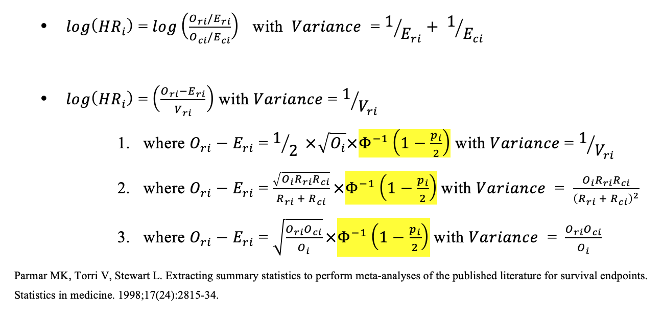
The accuracy and precision of the survival probabilities collected from the KM plots affect the accuracy and precision of the calculated hazard ratios during the use of Parmar's methodology and, in turn, determine the statistical significance of meta-analyses on hazard ratios. Traditionally, when collecting the survival probabilities from the KM plot, a researcher might use a ruler to locate certain coordinates on a printed KM plot. Alternatively, Guyot et al. [6] recommended using a general-purpose plot digitizer software, DigitizeIt [7], which functions as a digital ruler, to better extract the x and y values of the coordinates from a KM plot image file using an input device such as a mouse. However, it is laboriously difficult for a user, whether using a ruler or generalized software, to manually locate the coordinates one by one. More importantly, improvements could be made on traditional methods with respect to, firstly, the precision of a coordinate pointed out by a user and, secondly, the accuracy between the coordinate pointed out by a user and the coordinate intended by the user.
In the present study, SC2HR.py (Survival Curve To Hazard Ratio) is introduced as an open-source, all-in-one software tool written in the Python programming language [8]. All improvements for the scope of current studies stem from the idea of approaching the KM plot and Parmar's methodology at the pixel level. In order not to request information that requires an understanding of Parmar's methodology or Tierney's spreadsheet, SC2HR.py takes the strategy of requesting subsets of information that can be provided with routine knowledge of the KM plot (Fig. 1A). Then, SC2HR.py corrects user inputs to better recognize the KM plots in terms of precision and accuracy at the pixel level (Fig. 1B), and then allows the software to reconstruct information, which researchers traditionally had to provide based on their knowledge of Parmar's methodology, by letting the software enumerate survival curves from the origin on the x-axis to the right, pixel by pixel (Fig. 1C).
Figure 1. Overview of the pixel-level semi-automation of Parmar's methodology by SC2HR.py
(A) Without needing an understanding of Parmar's methodology, a researcher with routine knowledge of the KM plot can manually input information using a mouse or keyboard. This includes specifying an origin on the x-axis and an origin on the y-axis, a tick on each axis (with the y-axis tick, which specifically corresponds to a 1.0 survival probability), the numerical value of the tick on the x-axis, and the initial numbers of participants in the research and control groups, as well as the survival curves of both groups. (It is noted that this process may be easier than it appears after viewing Supplementary File S1. The numerical indices, such as "1101", "1102", "3001", etc., are used as per its patent application to minimize misidentification.)
(B) SC2HR.py corrects a coordinate selected by a user to the intended coordinate at the pixel level. This enhances the precision and accuracy of the information provided by the user.
(C) SC2HR.py automatically generates, in place of the user, the information necessary to compute a hazard ratio according to Parmar's methodology. Specifically, the "time interval" in SC2HR.py is programmed to be one pixel of the image file. This obviates the need for the user to manually select time intervals and then indicate the corresponding points on the survival curves.
2. Methods and Materials
2.1. Pixel-level Semi-automation of Parmar's Methodology (Figure 1)
2.1.1. Circumventing the Requirement of Understanding Parmar's Methodology (Figure 1A)
In traditional methods, such as using a ruler or general-purpose plot digitizer software like DigitizeIt [7], an understanding of Parmar's methodology is required, especially when selecting coordinates on the KM plot whose y-values are later converted to survival probabilities. More specifically, the process involves: first, dividing the x-axis, which represents time, into non-overlapping intervals or "time intervals" (not necessarily of equal length [2]), as depicted by the distance between imaginary vertical dotted lines in Figure 1C. Second, for each time interval from the origin on the x-axis to the right, the coordinate information of survival curves for control and research groups, represented as green and blue crosses, must be identified and marked, using either a pencil on a printed KM plot or the DigitizeIt software [7] on a digital image file [6]. Third, these y-values of coordinates should be computationally converted into survival probabilities, for input into Tierney's spreadsheet [5] or for manual calculation according to Parmar's methodology [2].
However, SC2HR.py has been designed to simplify the preparation steps, requiring only routine knowledge of KM plots. Firstly, SC2HR.py prompts the user to indicate four specific points on the KM plot using an input device (e.g., a mouse): origins on the x- and y-axes, a tick on the x-axis, and a tick on the y-axis corresponding to a 1.0 survival probability (Note: the origin on the x-axis may not always coincide with the origin on the y-axis on the KM plot). Secondly, the user is asked to enter the numerical value of the x-axis tick and the starting numbers of participants in the research and control groups. Thirdly, the user must indicate the survival curves of both groups using a mouse, as shown in the demonstration video (Supplementary File S1). In this way, SC2HR.py eliminates the need for the user to (i) determine the "time interval," (ii) locate coordinates of the research and control groups at the time intervals from the origin on the x-axis, and (iii) convert the y-values of the coordinates into survival probabilities.
2.1.2. Improving Accuracy and Precision in the Context of Parmar's Methodology (Figure 1B)
Whenever a user selects a specific spot on the KM plot, SC2HR.py searches for the nearest spots on KM plots based on the current context of information being requested, such as the origin of the coordinate or the survival curve of the control group. First, concerning the origins or ticks of the KM plots, SC2HR.py investigates the local minima in the funneling landscape of RGB values of pixels to find the intersection of the two lines nearby, aiming to enhance the precision and accuracy of acquiring the four points marked by a user to the pixel level. Second, for survival curves of either the control or research group, SC2HR.py is designed to collect the Y-values of survival curves, which are later computed into survival probabilities. For programmers, it's noteworthy that SC2HR.py reacts to the mouse's curve movement direction, focusing more on the horizontal or vertical aspects of nearby survival curves to capture information based on the user's mouse movement context.
2.1.3. Eliminating Manual Identification of Coordinates on Survival Curves (Figure 1C)
Traditionally, researchers had to manually identify several coordinates on the survival curves of the KM plots at the imaginary dotted lines representing non-overlapping time intervals. This method of manually and sparsely collecting information has been significantly improved by SC2HR.py, which is programmed to enumerate every pixel on the x-axis from the origin to the right, collecting as many y-values of survival curves of both research and control groups as possible. The narrower the time interval, the more information is gathered for computing a hazard ratio, aligning with Parmar's recommendation to choose time intervals that keep the event rate within the interval relatively small [2].
2.2. Evaluation
2.2.1. Accuracy and Precision of Corrected Coordinates
The accuracy of the coordinates corrected by SC2HR.py will be visually illustrated using a pixel-level magnifying-glass feature. For any specific mouse location, a pixel table with RGB values will be visually displayed on the right side of the GUI application. This feature magnifies the location pointed by the user and the location corrected by SC2HR.py, enabling a clear comparison.
Regarding precision, a specific point on the survival curves, measured by both DigitizeIt (a general-purpose plot digitizer software) and SC2HR.py, will be repeatedly measured to investigate the variance of measurements by SC2HR.py compared to DigitizeIt. This comparison reflects the degree of precision. Notably, both DigitizeIt and SC2HR.py require the coordinates of an origin on the X-axis, an origin on the Y-axis, a tick on the X-axis, and a tick on the Y-axis, along with the numerical value for the tick on the X-axis to calculate the value of the particular point (or, the tick on the X-axis). These steps will be repeated ten times for an F-test to determine whether the variance of SC2HR.py is lower than that of DigitizeIt.
Additionally, upon completing the steps required by SC2HR.py, a file named SC2HR.xlsx will be available, showcasing reconstructed pixel-level KM curves as perceived by SC2HR.py. More specifically and technically, SC2HR.py is programmed to consider that at least three pixels in a row must indicate the same Y-axis value, within a margin of error of +/- one pixel, before taking the Y-value into account for computing the survival probability according to Parmar's methodology. An uppercase "C" or "R" represents the pixel location identified by SC2HR.py where the Y-axis value remains exactly the same for three consecutive pixels. In contrast, a lowercase "c" or "r" represents a location where the Y-axis value deviates by just one pixel from a group of nearby pixels, such that adjusting that single "c" or "r" by one pixel would align all three Y-values for at least three consecutive times.
2.2.3. Verifying the Correctness of HR Computation Results
Censoring should be briefly mentioned. Censoring reflects amounts that cannot be accurately evaluated due to a lack of knowledge about what happened thereafter for reasons other than the outcome of interest (e.g., illness or death from other causes, withdrawal of consent, etc.) [9]. The appendix section of Parmar's methodology [2] proposed how to accommodate censoring to better estimate hazard ratios based on the assumption of a constant rate of censoring and the employment of minimum and maximum follow-up information (if available). Thus, with respect to the numerical dataset of Parmar et al. (pages 2825 ~ 2827), survival probabilities acquired from the KM plots using a mouse device will be used to compute hazard ratios and checked against the published hazard ratios.
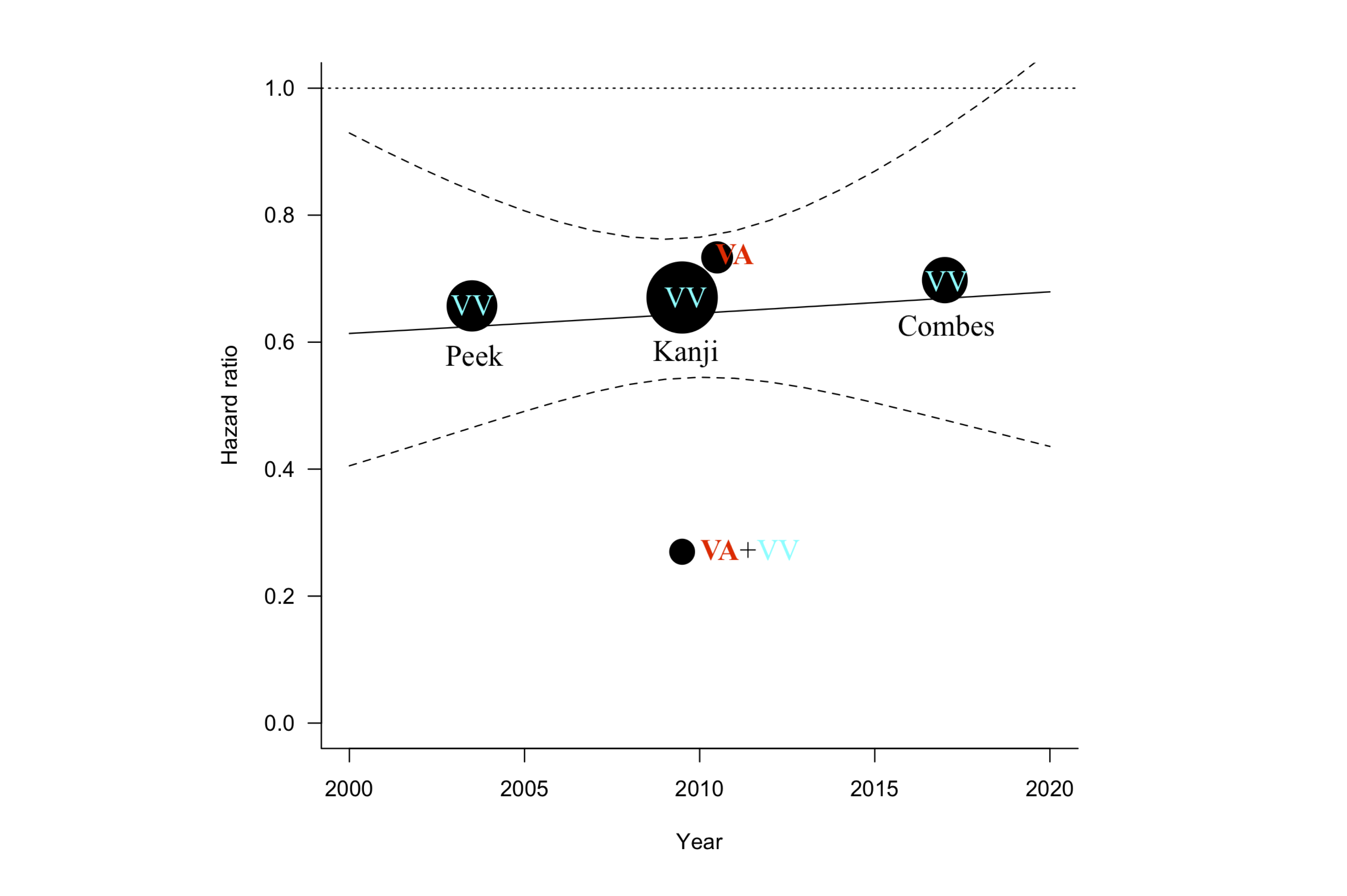
However, the constant rate-of-censoring assumption is not always the case, and the information of minimum and maximum follow-up in the trial tends to be unavailable. In fact, censoring is typically encountered and indirectly noticed when comparing the proportion of survival curves and the information in tables for the number of patients at risk at a given time (Supplemental Figure 2A), such that, to the best of our knowledge, the appendix section of Parmar's methodology cannot be applied for the purpose of testing the correctness of SC2HR.py against the published hazard ratios. In the meantime, Combes et al. published a KM survival curve [10] where the proportion of the survival curve matches the table of the number of patients at risk at a given time (Supplementary Figure 2B). Therefore, in this study, testing of SC2HR.py was performed for the dataset of Combes et al. [10], without applying the appendix part of Parmar's methodology to accommodate censoring [2].
Figure 2. Pixel-level correction
SC2HR.py enhances precision and accuracy by adjusting the coordinates selected by users. Given the challenges users face in pinpointing an exact location on an image with a mouse-like device to the precision of a single pixel, SC2HR.py automatically corrects the manually marked point (shown in red) to the intended point (shown in green).
>
3. Results
In terms of the accuracy of coordinates, SC2HR.py visually displays both the actual location marked by researchers and the corrected location intended by researchers at the pixel level. This feature allows for the visual verification of the pixel-level accuracy of the corrected locations, as illustrated in Figure 2. SC2HR.xlsx demonstrates the reconstructed pixel-level KM curves, showcasing how SC2HR.py interprets survival curves at the pixel level (Figure 3). The precision of SC2HR.py was compared against DigitizeIt by repeatedly measuring a specific point on a survival curve to observe the variability of each tool (Supplemental Data 3). Measurements taken with DigitizeIt software were as follows: (0.400, 98.0), (0.428, 98.1), (0.438, 97.7), (0.427, 98.2), (0.428, 98.1), (0.438, 98.0), (0.419, 98.2), (0.438, 97.9), (0.438, 97.9), (0.419, 98.0), and (0.438, 98.0). Measurements taken with SC2HR.py were: (0.433, 97.9), (0.433, 97.9), (0.433, 98.0), (0.426, 97.9), (0.419, 97.9), (0.433, 97.9), (0.426, 98.0), (0.426, 98.2), (0.426, 98.0), and (0.426, 97.9). The variances in X-values for DigitizeIt and SC2HR.py were 0.0001491 and 0.00002232, respectively, and the F-test results indicated that the variance of SC2HR.py was significantly lower than that of DigitizeIt (p = 0.00464). The variances in Y-values for DigitizeIt and SC2HR.py were 0.02178 and 0.00933, respectively; however, the F-test did not indicate a significant difference in variance between SC2HR.py and DigitizeIt for Y-values (p = 0.1114).
When testing SC2HR.py with the dataset from Parmar et al. [2] (Supplementary Data 3A), the computed log hazard ratio was XXXX, compared to -0.244 according to Parmar's computation [2] and -0.0235 in the original authors' report [2, 11], matching up to three decimal points. For the dataset from Combes et al. [10] (Supplementary Data 3B), SC2HR.py matched the reported hazard ratios up to the third decimal point, without applying the appendix part of Parmar's methodology.
SC2HR.xlsx illustrates the interpretation of survival curves at the pixel level by SC2HR.py. "C" and "c" denote the control group, while "R" and "r" represent the research group. Uppercase "C" or "R" indicates the pixel locations identified by SC2HR.py where the Y-axis value is consistent across three consecutive pixels. In contrast, lowercase "c" or "r" marks locations where the Y-axis value differs from the surrounding pixels by just one pixel. Adjusting this "c" or "r" by one pixel would align all three Y-values for at least three consecutive instances. The X-axis and Y-axis represent time and survival probabilities, respectively. For the X-axis, the first row displays the pixel-level location in the 10th digit, and the second row shows the index in the 1st digit. The third row indicates the time, computed based on the origin on the X-axis, the tick on the X-axis, and its value. Similarly, for the Y-axis, the first descriptive column under "===[...]===", labeled "Pixel," refers to the pixel-level location. The second column, labeled "Percent," represents the survival probability multiplied by 100. The third and fourth columns display the number of patients in the control and research groups at that specific pixel on the Y-axis, respectively.
4. Discussion
This study introduces SC2HR.py, an all-in-one software solution designed to enhance meta-analyses of time-to-event data. SC2HR.py allows researchers with basic knowledge of Kaplan-Meier (KM) plots to intuitively estimate hazard ratios from survival curves with improved precision and accuracy. Compared to previous general-purpose plot digitization software, SC2HR.py has demonstrated superior or at least equivalent precision in corrected coordinates, as validated by F-test results. Users of SC2HR.py can verify the accuracy of these coordinates themselves by consulting the pixel table displayed on the right side of the GUI application.
SC2HR.py's innovative approach to Parmar's methodology at the pixel level enables it to utilize general information about KM plots without requiring knowledge of Parmar's methodology. This facilitates the correction of user inputs for increased precision and accuracy at the pixel level and allows for the automatic construction of survival probabilities to apply Parmar's methodology. Thus, it eliminates the need for manually identifying coordinates on survival curves using a ruler or generic software, along with an understanding of Parmar's methodology.
Notably, this study does not propose modifications to Parmar's methodology itself but rather offers specialized software for the pixel-level semi-automation of this methodology, particularly enhancing the pre-processing phase of acquiring survival probabilities. The results can be verified against referenced values or using Tierney's spreadsheet, as discussed in the Results section. Furthermore, each line of open-source code relevant to Parmar's methodology has been written with readability in mind and peer-reviewed for correctness in terms of variable naming and process sequencing.
However, SC2HR.py has its limitations. Firstly, the default GUI size in version 1.0 is optimized for a 15-inch laptop monitor, suggesting that larger image files could potentially improve accuracy and precision in estimating hazard ratios. Nevertheless, Parmar has noted that published survival curves may be too small for accurate reading, indicating that simply enlarging the image might not be beneficial [2]. Secondly, the estimation of hazard ratios (HR) from a survival curve via SC2HR.py significantly depends on the collected survival probabilities, which in turn are contingent on the quality of the images, such as clarity and the scale of numerical axes [6]. Lastly, while the pixel-level semi-automation of Parmar's methodology addresses several issues within the scope of this study, further advancements in facilitating the conversion from KM plots to hazard ratios will require additional expertise in this domain.
Supplemental Figure 2. Censoring Issue and Applying the Constant Rate of Censoring Assumption
Censoring results from a lack of knowledge about what happens beyond the study endpoint for reasons unrelated to the outcome of interest. Parmar et al. proposed reflecting censoring by assuming a constant rate of censoring in their methodology's appendix section. However, since a constant rate of censoring often does not hold in real-life examples, and information on minimum and maximum follow-up in trials tends to be unavailable, applying the algorithm introduced in Parmar's appendix is typically not feasible.
(A) In practice, censoring is commonly encountered and can be indirectly observed when comparing the proportion of survival curves with the information in tables for the number of patients at risk at given times, which is often attributed to censoring. For instance, in the dataset and KM plot published by Takauji et al., at 10 hospital days, the survival probabilities for ECMO and Control groups - approximately 0.92 and 0.66, respectively - seem to correspond with the ratio of patients at risk to the initial patient numbers, 23/25=0.92 (A-1) and 59/89=0.66 (A-2). Conversely, at 50 hospital days, the survival probabilities for ECMO and Control groups, 0.6 and 0.34, do not align as expected with the ratios, 10/25=0.4 (A-3) and 16/89=0.18 (A-4), indicating the influence of censoring.
(B) In the absence of censoring, the proportions derived from survival curves should match the information in tables for the number of patients at risk at a given time. In the KM survival curve from Combes et al., at 50 hospital days, the survival probabilities for ECMO and control groups, 0.67 and 0.58, closely match the ratios of patients at risk to the initial patient numbers, 83/124=0.67 (B-3) and 72/125=0.58 (B-4). Therefore, for the dataset from Combes et al., SC2HR.py was tested without applying the algorithm introduced in the Appendix section of Parmar's methodology.
5. Conclusion
SC2HR.py is designed to facilitate the estimation of hazard ratios from survival curves by providing a GUI environment in which users with basic knowledge of KM plots can intuitively input information necessary for the integrated computer system to employ Parmar's methodology. This enhancement in the accuracy and precision of user input recognition, and consequently in hazard ratio estimates, positions SC2HR.py alongside several prior efforts aimed at streamlining Parmar's methodology. By equipping researchers with a tool that incorporates different developers' perspectives, SC2HR.py enhances confidence in analyzing and reporting hazard ratios and their variances.
Software Instruction in Relation to Patent Application
Installation
After installing the latest version of Python (version 3.x or greater) on your operating system, please open SC2HR.py using Python's Integrated Development and Learning Environment (IDLE). To install the required Python libraries such as PIL, numpy, and openpyxl, you can open a terminal window and type the following commands:
sudo pip3.8 install Pillow
sudo easy_install-3.8 numpy
sudo easy_install-3.8 openpyxl
Python IDLE allows you to execute SC2HR.py by pressing the F5 button or selecting "Run Module" from the menu. The Graphical User Interface (GUI) of SC2HR.py will then be displayed on your monitor. The GUI is divided into two parts: the left part, known as a canvas, where the Kaplan-Meier survival curve image file will be loaded, and the right part, which contains two tabs. The 'Step' tab highlights the current instruction step in red font; completing a step de-highlights it and highlights the next step. The 'Pixel' tab, functioning like a magnifying-glass feature, displays both the actual location marked by a researcher and the corrected location intended by the researcher at the pixel level. Users can manually select one of these tabs, but the relevant tab for the current stage of Parmar's methodology will be automatically chosen as needed.
To START, click the beige canvas on the left.
Upon first executing SC2HR.py, this instruction will be highlighted in yellow with the font in reddish bold. Please click on the beige-colored part of the GUI on the left, which will open a pop-up directory folder. Select your graphical image of the Kaplan-Meier plot in file extension formats 'png', 'jpg', or 'gif'.
An origin on the x-axis (1101) => A tick on the x-axis (1102)
On the loaded Kaplan-Meier survival curve image, mark the origin on the X-axis by clicking and holding (mouse-down) and then mark the largest tick on the X-axis by releasing the mouse button (mouse-up).
A tick on the y-axis (1103) => An origin on the y-axis (1104)
Similarly, mark the tick on the Y-axis that represents a survival probability of 1.0 by clicking and holding (mouse-down) and then mark the origin on the Y-axis by releasing the mouse button (mouse-up). Concentric circles will appear at the X-coordinate of the origin on the X-axis and the Y-coordinate of the tick on the Y-axis.
Survival curve@Control (1105)
Mark the survival curve of the control group by pressing and holding the mouse button from the center of the concentric circles to the end of the curve.
Survival curve@Research (1106)
Similarly, mark the survival curve of the research group by continuing to press down all the way.
Fill in the following forms:
Type in the number of patients in the research and control groups in "Effective number@Control" and "Effective number@Research", respectively, representing the "effective number alive at the start of the time interval." Fill in the entry for "Tick@X-axis," which requires the largest number indicating the rightmost tick on the X-axis.
FOR ANALYSIS, click the previous canvas on the left
Clicking the canvas on the left side of the GUI will save the output in SC_output.xlsx, and log information will be available in the Python shell.
[Result] ln(HR): 0.0, ln(variance): 0.0
The estimated natural log of the HR and log variance from the Kaplan-Meier plot will then be available.
Reference
1. Smith, C.T. Meta-analysis of time-to-event data. 2018 [cited 2019 March, 29th]; Available from: https://training.cochrane.org/resource/meta-analysis-time-event-data.
2. Parmar, M.K., V. Torri, and L. Stewart, Extracting summary statistics to perform meta-analyses of the published literature for survival endpoints. Stat Med, 1998. 17(24): p. 2815-34.
3. Chu, D.K., et al., Mortality and morbidity in acutely ill adults treated with liberal versus conservative oxygen therapy (IOTA): a systematic review and meta-analysis. Lancet, 2018. 391(10131): p. 1693-1705.
4. Roh, H.F., et al., Pulmonary resection for patients with multidrug-resistant tuberculosis based on survival outcomes: a systematic review and meta-analysis. Eur J Cardiothorac Surg, 2017. 52(4): p. 673-678.
5. Tierney, J.F., et al., Practical methods for incorporating summary time-to-event data into meta-analysis. Trials, 2007. 8: p. 16.
6. Guyot, P., et al., Enhanced secondary analysis of survival data: reconstructing the data from published Kaplan-Meier survival curves. BMC Med Res Methodol, 2012. 12: p. 9.
7. Bormann, I. Digitizer software - digitize a scanned graph or chart into (x,y)-data.; Available from: http://www.digitizeit.de/.
8. Foundation, P.S. Welcome to Python.org. Available from: https://www.python.org.
9. Rich, J.T., et al., A practical guide to understanding Kaplan-Meier curves. Otolaryngol Head Neck Surg, 2010. 143(3): p. 331-6.
10. Combes, A., et al., Extracorporeal Membrane Oxygenation for Severe Acute Respiratory Distress Syndrome. N Engl J Med, 2018. 378(21): p. 1965-1975.
11. Ingle, J.N., et al., Randomized trial of tamoxifen alone or combined with aminoglutethimide and hydrocortisone in women with metastatic breast cancer. J Clin Oncol, 1986. 4(6): p. 958-64.
12. Tierney, J.F., et al., Response to: Practical methods for incorporating summary time-to-event data into meta. Authors' reply. Trials, 2013. 14: p. 391.
13. Takauji, S., et al., Respiratory extracorporeal membrane oxygenation for severe sepsis and septic shock in adults: a propensity score analysis in a multicenter retrospective observational study. Acute Med Surg, 2017. 4(4): p. 408-417.
14. Hoyle, M.W. and W. Henley, Improved curve fits to summary survival data: application to economic evaluation of health technologies. BMC Med Res Methodol, 2011. 11: p. 139.
15. Pocock, S.J., T.C. Clayton, and D.G. Altman, Survival plots of time-to-event outcomes in clinical trials: good practice and pitfalls. Lancet, 2002. 359(9318): p. 1686-9.
Note:
As long as this article and the name of the trademark are formally and reasonably referred to, and as long as a user accepts the license agreement form (https://ngene.org/download.html), it will be an honor for the source code being openly employed by the public to contribute to accelerating the advancements in the methodology of meta-analysis and relevant fields.
SCI-Indexed Scripts
[R: Logistic-based Systolic Model Simulation, Parameter Estimation, and Spearman/Kendall-correlation]
Per the International Classification of Diseases, Tenth Revision (ICD-10), "Other Hyperlipidemia" is classified under the code E784. The code E1329 is assigned to "Other Specified Diabetes Mellitus with Other Diabetic Kidney Complication." Additionally, J9699 refers to "Respiratory Failure, Unspecified, Type Unspecified."
In addition, the above Python script is designed to extract data from the file icd10cm_tabular_2024.xml obtained from the official website of the Centers for Medicare & Medicaid Services (CMS). The primary function of this script is to efficiently process the extracted data for the creation of the file CMS_ICD10.js.
ABGA-Based Acid–Base & Anion‐Gap Monitor for Ventilation & Dialysis
Acid-Base Imbalances and Their Management in Ventilation and Hemodialysis
Fundamentals of Acid-Base Balance
The human body requires a tightly regulated blood pH (around 7.40) for optimal cellular function. Acid-base balance is maintained by buffering systems and by the coordinated function of the lungs and kidneys. The major buffer in the blood is the bicarbonate–carbonic acid system: carbon dioxide (CO 2 ) produced by metabolism is converted to carbonic acid (H 2 CO 3 ) in blood, which dissociates into hydrogen ions (H + ) and bicarbonate (HCO 3 – ). The lungs regulate the level of CO 2 (an acidic component) through ventilation, while the kidneys regulate HCO 3 – (a basic component) through reabsorption and excretion of bicarbonate and hydrogen ions. Together, these mechanisms keep the arterial pH in a narrow normal range (approximately 7.35–7.45).
The quantitative relationship between CO 2 , bicarbonate, and pH is described by the Henderson–Hasselbalch equation: \( \mathrm{pH} = 6.1 + \log\frac{[\text{HCO}_3^-]}{0.03 \times \mathrm{PaCO_2}} \). This equation highlights that blood pH is determined by the ratio of bicarbonate (metabolic component) to carbonic acid (reflecting PaCO 2 , the respiratory component). Because pH is a logarithmic scale of H + concentration, small changes in pH denote large changes in [H + ]. At the normal pH of 7.40, the [H + ] is about 40 nmol/L; if pH drops to 7.10, [H + ] rises to ~80 nmol/L (doubling the hydrogen ion concentration for a 0.3 unit pH decrease). Thus, even mild derangements in pH can have significant physiological effects, and larger deviations (pH < 7.20 or > 7.60) can be life-threatening.
Arterial Blood Gas (ABG) analysis is a fundamental test to assess a patient’s acid-base status and oxygenation. An ABG directly measures blood pH, PaCO 2 , and PaO 2 , and reports calculated values like HCO 3 – (derived from the measured pH and PaCO 2 ) and base excess. The table below summarizes the key parameters and their normal reference ranges in arterial blood. “Base excess” indicates the amount of excess or deficient base in the blood: a negative base excess (also called a base deficit) indicates a deficit of base (consistent with metabolic acidosis), while a positive base excess indicates an excess of base (consistent with metabolic alkalosis). The anion gap, though not part of a standard ABG printout, is a calculated value using electrolyte measurements that aids in categorizing metabolic acidosis. With these values, clinicians can determine whether an acidosis or alkalosis is present and discern if the primary cause is respiratory or metabolic.
Parameter
Normal Range
Description
Arterial pH
7.35 – 7.45
Balance between acids and bases in blood
PaCO
2
35 – 45 mmHg
Partial pressure of carbon dioxide (acid component)
HCO
3–
22 – 26 mEq/L
Bicarbonate concentration (base component)
Base Excess
–2 to +2 mEq/L
Calculated excess or deficit of base in blood
Anion Gap
8 – 12 mEq/L
Difference between primary cations and anions; indicates unmeasured ions
PaO
2
75 – 100 mmHg
Partial pressure of oxygen (for context, not directly for acid-base)
O
2
Saturation
95 – 100%
Hemoglobin oxygen saturation (for context)
Approach to Acid-Base Disorders
A systematic approach to interpreting ABG results is crucial for accurately diagnosing the type of acid-base disturbance and guiding appropriate management.
Determine the blood pH to identify
acidemia
(pH < 7.35) or
alkalemia
(pH > 7.45).
Identify the primary disturbance by analyzing PaCO
2
and HCO
3–
:
If pH is low (acidemia): an elevated PaCO
2
indicates primary
respiratory acidosis
, whereas a low HCO
3–
indicates primary
metabolic acidosis
.
If pH is high (alkalemia): a low PaCO
2
indicates primary
respiratory alkalosis
, whereas a high HCO
3–
indicates primary
metabolic alkalosis
.
If pH is near normal (7.35–7.45) but other values are abnormal, a mixed disorder may be present (e.g., combined acidosis and alkalosis balancing out).
Assess whether the respiratory component is acute or chronic (if applicable):
In acute respiratory disorders, renal compensation is minimal; in chronic disorders, renal compensation adjusts HCO
3–
significantly.
For example, an acute rise in PaCO
2
causes a small HCO
3–
increase (~1 mEq/L per 10 mmHg PaCO
2
above 40), while chronic elevation causes a larger increase (~3–4 mEq/L per 10 mmHg).
Calculate the expected compensatory response for the primary disorder:
Metabolic Acidosis:
Use Winter’s formula to estimate expected respiratory compensation: \( \text{Expected PaCO}_2 = 1.5 \times [\text{HCO}_3^-] + 8 \pm 2 \) mmHg.
Metabolic Alkalosis:
Expected respiratory compensation: \( \text{Expected PaCO}_2 = 0.7 \times [\text{HCO}_3^-] + 20 \pm 5 \) mmHg (typically, PaCO
2
will rise, but usually not above ~55 mmHg).
Respiratory Acidosis:
Expected renal compensation: acute – HCO
3–
increases ~1 mEq/L for each 10 mmHg PaCO
2
above 40; chronic – HCO
3–
increases ~3–4 mEq/L per 10 mmHg.
Respiratory Alkalosis:
Expected renal compensation: acute – HCO
3–
decreases ~2 mEq/L for each 10 mmHg PaCO
2
below 40; chronic – HCO
3–
decreases ~4–5 mEq/L per 10 mmHg.
Compare the patient’s actual values to the expected compensation:
If the measured PaCO
2
or HCO
3–
is outside the expected range, suspect a
mixed acid-base disorder
. For example, an inappropriately high PaCO
2
in metabolic acidosis suggests an additional respiratory acidosis.
The body never overcompensates; a normalized pH in an ill patient often indicates mixed disorders.
If metabolic acidosis is present, calculate the
anion gap (AG)
:
AG = [Na
+
] – ([Cl
–
] + [HCO
3–
]). A normal AG is ~8–12 mEq/L (assuming normal albumin).
High anion gap acidosis
suggests addition of unmeasured acids (e.g. lactate, ketones, toxins).
Normal anion gap acidosis
(hyperchloremic) suggests HCO
3–
loss or H
+
retention (e.g. diarrhea or renal tubular acidosis).
If AG is elevated, calculate the delta ratio: \( \Delta = \frac{\text{AG} - 12}{24 - [\text{HCO}_3^-]} \). This helps detect mixed metabolic disorders (for example, Δ > 2 may indicate a concurrent metabolic alkalosis, while Δ < 1 suggests an additional normal-AG acidosis).
Interpret the results in clinical context to identify the underlying cause and initiate appropriate intervention for the patient.
Note:
A stepwise approach to ABG interpretation ensures that no aspect of the disorder is overlooked. Always consider the clinical picture – numbers must be correlated with the patient’s symptoms and history.
Respiratory Acid-Base Disorders
Respiratory disorders are caused by primary changes in PaCO 2 due to altered ventilation. These conditions can be acute or chronic, and the distinction is important because the body’s renal compensatory response takes time (days) to develop fully in chronic cases.
Respiratory Acidosis
Definition: Respiratory acidosis is characterized by elevated PaCO 2 (hypercapnia) and a reduced blood pH. It occurs when alveolar ventilation is inadequate relative to CO 2 production.
Common Causes: Anything that causes hypoventilation can lead to respiratory acidosis. Examples include obstructive lung diseases (such as chronic obstructive pulmonary disease, asthma exacerbation), respiratory muscle fatigue or paralysis (e.g. neuromuscular disorders like myasthenia gravis, Guillain-Barré syndrome), central respiratory depression (due to sedative or opioid overdose), or airway obstruction. In acute cases like drug-induced respiratory arrest, CO 2 rises rapidly; in chronic cases like COPD, kidneys retain bicarbonate to compensate.
Acute vs Chronic: In acute respiratory acidosis, the pH drops significantly with a small rise in HCO 3 – (because renal compensation is minimal initially). In chronic respiratory acidosis, the kidneys increase HCO 3 – reabsorption and generate buffers, so pH is closer to normal (partial compensation). For instance, an acute PaCO 2 of 60 mmHg may yield HCO 3 – ~26 mEq/L, whereas chronically the HCO 3 – might be ~30 mEq/L.
Mathematical Insight: The relationship between CO 2 and pH is given by the Henderson–Hasselbalch equation: \( \text{pH} = 6.1 + \log\frac{[\text{HCO}_3^-]}{0.03 \times \text{PaCO}_2} \). In respiratory acidosis, PaCO 2 is elevated, driving the equation toward a lower pH unless HCO 3 – increases accordingly. This can also be viewed in terms of [H + ]: \( [H^+] (\text{nM}) \approx 24 \times \frac{\text{PaCO}_2}{[\text{HCO}_3^-]} \). As PaCO 2 rises, [H + ] increases (and pH drops) unless buffered by HCO 3 – .
Clinical Effects: Elevated CO 2 levels cause headache, confusion, and can depress consciousness (CO 2 narcosis) in severe cases. The respiratory drive may be blunted in chronic hypercapnia (e.g., in CO 2 retainers like COPD patients, who rely on hypoxic drive).
Management: The primary treatment is to improve ventilation. Depending on severity, this may involve stimulating the patient to breathe, reversing sedatives, or providing assisted ventilation (e.g. non-invasive ventilation like BiPAP or mechanical ventilation). Oxygen is provided cautiously in chronic CO 2 retainers to avoid wiping out the hypoxic respiratory drive. In life-threatening acute respiratory acidosis, endotracheal intubation and controlled ventilation may be necessary to quickly reduce PaCO 2 . Hemodialysis has a limited role in pure respiratory acidosis because it does not efficiently remove CO 2 ; the focus is on ventilatory support. Underlying causes should be addressed concurrently (e.g., bronchodilators for asthma, antidotes for drug overdose).
Respiratory Alkalosis
Definition: Respiratory alkalosis is characterized by low PaCO 2 (hypocapnia) and an elevated blood pH. It results from excessive alveolar ventilation (hyperventilation) relative to CO 2 production.
Common Causes: Any trigger of hyperventilation can cause respiratory alkalosis. Common causes include anxiety or panic attacks (psychogenic hyperventilation), pain, fever, pregnancy (increased respiratory drive), stimulant drug use, and hypoxemia-driven hyperventilation (as in pulmonary embolism or high altitude). Iatrogenic causes include excessive mechanical ventilation. Some conditions like early salicylate overdose and sepsis can also stimulate hyperventilation.
Acute vs Chronic: Acute respiratory alkalosis (e.g., during a panic attack) shows an increase in pH with a slight reduction in HCO 3 – (renal compensation hasn’t had time to occur). Chronic respiratory alkalosis (e.g., in high-altitude residents or pregnancy) leads to a more sustained bicarbonate drop as kidneys excrete HCO 3 – over days. For example, an acute PaCO 2 of 25 mmHg might bring HCO 3 – down to ~20 mEq/L acutely, whereas chronically it could fall further to ~17–18 mEq/L.
Clinical Effects: Symptoms of acute respiratory alkalosis include lightheadedness, tingling in the extremities or around the mouth (paresthesias), and sometimes muscle cramps or even fainting. Severe alkalosis can induce tetany or seizures due to decreased ionized calcium. Chronic cases are often asymptomatic as metabolic adjustments occur.
Management: The key is to address the cause of hyperventilation. If due to anxiety, calming techniques or mild sedatives can help (for example, coaching controlled breathing or having the patient breathe into a rebreathing device to increase CO 2 ). In pain or fever, treat those underlying issues. For patients on mechanical ventilators, settings should be adjusted to reduce minute ventilation (lower tidal volume or rate) to correct alkalosis. In extreme cases where pH > 7.60 and symptoms are severe, careful sedation or temporary neuromuscular blockade (with controlled ventilation) might be used to prevent dangerous consequences of hyperventilation. Dialysis has no direct role in treating respiratory alkalosis; the focus is on reducing ventilation to allow CO 2 levels to return toward normal. Throughout treatment, ensure adequate oxygenation even as you moderate the ventilation.
Metabolic Acid-Base Disorders
Metabolic disorders stem from primary changes in bicarbonate or the addition/removal of acids from the body. They often involve the kidneys, gastrointestinal tract, or systemic metabolic processes. Respiratory compensation (changes in ventilation to adjust PaCO 2 ) occurs rapidly in metabolic disorders, but definitive correction usually requires addressing the underlying metabolic cause or using interventions like fluids, medications, or dialysis.
Metabolic Acidosis
Definition: Metabolic acidosis is defined by reduced HCO 3 – and a low pH. This results from either an accumulation of acids or a loss of bicarbonate from the body.
Classification by Anion Gap: It is crucial to determine if the metabolic acidosis has a high anion gap (AG) or a normal anion gap.
High Anion Gap Metabolic Acidosis (HAGMA):
Occurs when excess acids add unmeasured anions, raising the AG above normal (> 12 mEq/L). Common causes can be remembered by the mnemonic
MUDPILES
(Methanol, Uremia (renal failure), Diabetic ketoacidosis, Propylene glycol/Paraldehyde, Iron/INH (isoniazid), Lactic acidosis, Ethylene glycol, Salicylates). Lactic acidosis (from shock or severe hypoperfusion), ketoacidosis (due to diabetes, alcoholism, or starvation), and uremic acidosis (advanced renal failure) are frequent high-AG causes.
Normal Anion Gap Metabolic Acidosis (NAGMA):
Also known as hyperchloremic acidosis, occurs when bicarbonate is lost but replaced by chloride, so the AG remains normal. Typical causes include gastrointestinal bicarbonate loss (severe diarrhea, ileostomy drainage), renal bicarbonate loss (renal tubular acidosis), or ingestion/infusion of H
+
or NH
4+
(such as ammonium chloride administration).
Physiological Effects: Significant acidemia (especially when pH < 7.20) can impair cardiac contractility, predispose to arrhythmias, and cause vasodilation and hypotension. Patients with metabolic acidosis often exhibit Kussmaul respirations (deep, rapid breathing) as a compensatory mechanism to blow off CO 2 . Additionally, acidosis causes potassium to shift out of cells, often leading to hyperkalemia (although total body potassium may be depleted in conditions like diabetic ketoacidosis).
Key Equations: Metabolic acidosis is reflected by a decrease in the bicarbonate level in the Henderson–Hasselbalch relationship. The expected respiratory compensation can be calculated by Winter’s formula: \( \text{Expected PaCO}_2 = 1.5 \times [\text{HCO}_3^-] + 8 \pm 2 \). For example, if HCO 3 – is 12 mEq/L, the expected PaCO 2 ≈ 1.5(12) + 8 = 26 mmHg (±2). If the actual PaCO 2 is significantly higher than this (in the 30s or 40s), it indicates a concomitant respiratory acidosis (i.e. ventilatory failure to compensate); if it is much lower (in the teens), a respiratory alkalosis is also present. The anion gap formula is \( \text{AG} = [\text{Na}^+] - ([\text{Cl}^-] + [\text{HCO}_3^-]) \), which helps identify HAGMA. In HAGMA, comparing the increase in AG to the decrease in HCO 3 – (the delta ratio) can uncover mixed disorders. As a guideline, if \( \Delta = \frac{\text{AG} - 12}{24 - [\text{HCO}_3^-]} \) exceeds 2, it suggests an additional metabolic alkalosis; if Δ is below 1, it suggests an additional normal-AG metabolic acidosis on top of the high-AG process.
Management: The cornerstone of treatment is addressing the underlying cause of acidosis.
In diabetic ketoacidosis (DKA), administer insulin and IV fluids, which will resolve ketoacid production and gradually correct the acidosis. Potassium supplementation is essential as insulin drives K
+
back into cells.
In lactic acidosis, improve tissue perfusion and oxygenation (treat shock or cardiac failure, give oxygen, and address any sepsis or underlying cause of the lactic acidosis).
For renal failure (uremia) or toxic alcohol/poisoning-induced acidosis (e.g., methanol or ethylene glycol ingestion, or severe salicylate overdose), urgent
hemodialysis
is often indicated to remove acids or toxins and correct the acid-base disturbance.
For severe metabolic acidosis (typically pH < 7.1) of any cause, intravenous sodium bicarbonate can be considered as a temporary measure to improve pH. This is used cautiously, as it can cause sodium load, volume overload, and paradoxical CO
2
generation; it is most appropriate when acidosis is extreme or when waiting for other therapies to take effect.
Throughout management, respiratory support is crucial. Patients may tire from hyperventilation. Mechanical ventilation can be used to support breathing and control PaCO 2 , buying time while metabolic treatment takes effect. For example, in severe DKA or sepsis, if the patient is in respiratory failure or exhausting from respiratory effort, a ventilator can maintain ventilation to keep the pH in a safe range. Meanwhile, if the acidosis is primarily due to renal failure or an ingested toxin and is not rapidly reversible, dialysis provides definitive correction by removing acid load and restoring electrolyte balance. Careful monitoring of ABG values and electrolytes (especially potassium) is necessary during treatment, as correcting acidosis will cause K + to shift back into cells, potentially precipitating hypokalemia if not managed.
Metabolic Alkalosis
Definition: Metabolic alkalosis is marked by elevated HCO 3 – and a high pH. It arises from an excess of base or a loss of acid from the body, and it is often associated with volume contraction and electrolyte disturbances.
Common Causes: The causes of metabolic alkalosis are often categorized based on chloride responsiveness and volume status.
Chloride-responsive alkalosis:
(Urine Cl
–
< 20 mEq/L) Usually due to loss of gastric acid (prolonged vomiting or nasogastric suction) or thiazide/loop diuretic use. These lead to volume contraction and chloride depletion; patients often have low blood chloride and respond to saline infusion (hence termed “saline-responsive”). Contraction alkalosis (from volume loss) and post-hypercapnia alkalosis (after rapid correction of chronic high CO
2
) also fall in this category.
Chloride-resistant alkalosis:
(Urine Cl
–
> 20 mEq/L) Caused by states of mineralocorticoid excess or severe potassium depletion. Examples include primary hyperaldosteronism (Conn’s syndrome), Cushing’s syndrome, prolonged excessive ingestion of bicarbonate (with renal impairment), or profound K
+
deficiency. In these cases, high aldosterone levels or low K
+
result in renal H
+
loss and bicarbonate retention; the alkalosis persists even with normal saline (hence saline-unresponsive).
Physiological Effects: Alkalemia can cause confusion, muscle twitching, and predispose to arrhythmias (especially in the presence of accompanying hypokalemia). It shifts the oxygen-hemoglobin dissociation curve to the left, which can impair oxygen delivery to tissues. Patients might have weakness or muscle cramps; severe alkalosis (pH > 7.55–7.60) can lead to neuromuscular irritability (tetany) and seizures.
Compensation: The respiratory system compensates by hypoventilation to raise PaCO 2 . However, hypoventilation is limited by the body’s need for adequate oxygenation. Generally, for each 1 mEq/L rise in HCO 3 – , PaCO 2 increases by ~0.5–0.7 mmHg. An estimation formula for expected compensation is: \( \text{Expected PaCO}_2 = 0.7 \times [\text{HCO}_3^-] + 20 \pm 5 \). For instance, if HCO 3 – is 36 mEq/L, the expected compensatory PaCO 2 would be around 0.7(36) + 20 ≈ 45 mmHg. In practice, the PaCO 2 in metabolic alkalosis rarely rises above 55–60 mmHg, as hypoventilation is limited by hypoxic drive.
Management: Treatment focuses on correcting the underlying cause and restoring volume and electrolyte balance.
For chloride-responsive alkalosis (e.g., due to vomiting or diuretic use): administer IV saline (to correct volume and chloride depletion) and replace potassium if low. This allows the kidneys to excrete bicarbonate (since volume repletion and chloride are restored). Potassium supplementation is especially important because hypokalemia both causes and maintains alkalosis (low K
+
leads to H
+
shifting into cells and increased renal H
+
loss).
For chloride-resistant alkalosis (e.g., primary hyperaldosteronism or severe hypokalemia): address the hormonal excess (e.g., adrenal tumor resection or use of aldosterone antagonists like spironolactone) and aggressively replete potassium. If the patient is hypertensive due to hyperaldosteronism, spironolactone or eplerenone can both treat the hypertension and help correct the alkalosis by blocking aldosterone’s effect.
If metabolic alkalosis is severe (pH > 7.60) or causing significant symptoms (e.g., arrhythmias or neurologic symptoms) and the above measures are insufficient or not feasible, more aggressive interventions can be used. These include administration of acid (such as dilute HCl infusion in a central line) or initiating dialysis with an acidified dialysate (particularly if the patient has renal failure or cannot tolerate large volumes of fluids).
During treatment of metabolic alkalosis, ventilation should not be excessively suppressed to dangerous levels. If the patient is on mechanical ventilation, avoid setting a respiratory rate that is too low, which could lead to hypoxemia. The ventilator can be adjusted to maintain adequate oxygenation and a modestly elevated PaCO 2 (permissive hypercapnia) to help gradually correct the alkalosis. In refractory cases or if the patient is already on dialysis for kidney failure, hemodialysis can be used to rapidly adjust bicarbonate levels by choosing an appropriate dialysate composition. Careful monitoring is needed to prevent over-correction and to manage electrolytes, especially potassium.
Conclusion
Acid-base imbalances encompass a range of disorders that can significantly impact patient outcomes if not recognized and treated promptly. A solid understanding of the underlying physiology and a stepwise analytical approach is essential for healthcare providers managing these conditions. By utilizing arterial blood gas data, mathematical tools (like compensation formulas and anion gap calculations), and correlating the results with the clinical scenario, one can accurately diagnose whether an acidosis or alkalosis is respiratory, metabolic, or mixed in origin. From there, appropriate interventions are chosen: ventilatory support for disturbances involving CO 2 (and as supportive therapy in severe metabolic derangements) and hemodialysis or targeted medical treatments for metabolic disturbances (especially those due to renal failure or toxin accumulation). Ultimately, managing acid-base disorders often requires a multidisciplinary approach — addressing the immediate pH imbalance while treating root causes — to restore the patient’s internal equilibrium and ensure the best possible outcome.
Written on July 20, 2025
The Importance of Anion Gap in Mechanically Ventilated Patients
Critically ill patients on mechanical ventilators often present with complex acid–base disturbances. While the ventilator can control carbon dioxide levels (respiratory component of pH), underlying metabolic abnormalities may still occur and can be less apparent from pH alone. The anion gap is a vital diagnostic tool in this context, helping clinicians identify and differentiate metabolic acidosis in ventilated patients. By analyzing the anion gap, one can determine whether a metabolic acidosis is present and classify it as either high anion gap or normal anion gap . This distinction guides the differential diagnosis—high anion gap acidosis typically indicates the accumulation of unmeasured acidic anions (often in life-threatening conditions), whereas normal anion gap acidosis suggests a loss of bicarbonate or retention of chloride. In a ventilated patient, recognizing a raised anion gap is crucial: it may reveal a serious metabolic problem (such as lactic acidosis or diabetic ketoacidosis) that requires urgent intervention, even if the blood pH is being partially compensated by the ventilator settings.
I. Anion Gap: Definition and Calculation
The anion gap (AG) is a calculated value representing the difference between measured cations (positively charged ions) and measured anions (negatively charged ions) in the blood. It reflects the quantity of unmeasured anions present. Under normal circumstances, the body maintains electroneutrality: the sum of positive charges equals the sum of negative charges. However, only a few major ions are routinely measured in standard laboratory tests. The anion gap is computed to estimate the “missing” ions in this balance.
In clinical practice, the anion gap is commonly calculated from serum electrolytes using the formula:
where [Na + ] is sodium, [K + ] is potassium, [Cl − ] is chloride, and [HCO 3 − ] is bicarbonate, all in mmol/L. Some laboratories omit potassium in this formula (because K + is usually low in concentration); in such cases the formula simplifies to AG = [Na + ] - ([Cl - ] + [HCO 3 - ]) . Whether potassium is included or not, the concept remains the same.
Normal values: A normal anion gap (with potassium included) is roughly 12 ± 4 mEq/L. If potassium is excluded, the normal range is a bit lower (around 8–12 mEq/L). The exact “normal” value varies with laboratory and patient conditions. Importantly, the normal anion gap depends on the level of serum albumin, the major unmeasured anion in blood. Albumin adjustment: For each 1 g/dL decrease in albumin (below the normal ~4 g/dL), the normal AG value drops by about 2.5 mEq/L. This means that a critically ill patient with hypoalbuminemia can have a deceptively low measured anion gap even in the presence of unmeasured acids. Clinicians often correct the anion gap for albumin to improve accuracy. The corrected anion gap can be estimated as:
using albumin in g/dL. For example, if albumin is 2 g/dL, the correction adds roughly 5 mEq/L to the calculated AG. This adjustment is often worthwhile in ICU patients, since many are hypoalbuminemic; it ensures that a high anion gap metabolic acidosis is not missed due to a low albumin level masking the gap.
Interpretation: In a healthy individual, the major measured cation (sodium) slightly exceeds the measured anions (chloride and bicarbonate), yielding a small gap (~10–12 mEq/L) which is accounted for by unmeasured anions (primarily albumin, phosphates, sulfates, and organic acids). An elevated anion gap indicates an excess of unmeasured anions in the blood, suggesting the presence of metabolic acidosis due to acids like lactate, ketones, or toxins. A normal anion gap in the face of metabolic acidosis implies that the drop in bicarbonate is counterbalanced by an increase in chloride (the other measured anion), meaning no significant accumulation of unmeasured anions has occurred. Both scenarios are discussed below. It is important to always evaluate the anion gap in any ventilated patient who has a low bicarbonate or acidemia, because the ventilator can adjust CO 2 and potentially mask the usual respiratory signs of a metabolic acidosis. An unexpected high anion gap should be treated as a red flag for serious underlying conditions requiring prompt investigation.
II. High Anion Gap Metabolic Acidosis
A high anion gap metabolic acidosis (HAGMA) occurs when there is an accumulation of acids that are not captured among the routinely measured electrolytes. In these cases, bicarbonate is consumed (buffering the excess H + from the acid) and the conjugate base of that acid (an unmeasured anion) accumulates, increasing the anion gap. The presence of a high anion gap in a ventilated patient is especially significant, as it often points to conditions that are potentially life-threatening and require prompt diagnosis and management. Common causes of HAGMA include:
Lactic Acidosis:
Lactic acidosis is one of the most frequent causes of a high anion gap in critically ill patients. It results from an overproduction or impaired clearance of lactic acid, typically due to tissue hypoperfusion or hypoxia. When cells lack adequate oxygen (as in septic shock, cardiogenic shock, or severe hypoxemia), they switch to anaerobic metabolism, producing lactic acid. The lactic acid dissociates into lactate
−
(an unmeasured anion) and H
+
, leading to a drop in bicarbonate as the H
+
is buffered, and a rise in the anion gap. Clinically, a ventilated patient with lactic acidosis may have low blood pressure, poor peripheral perfusion, or other signs of shock/sepsis. The anion gap is critical here: a rising gap can be an early indicator of worsening tissue hypoxia and lactic acid buildup, even if pH is partially maintained by ventilation.
Management:
Addressing lactic acidosis involves treating its root cause—improving oxygen delivery and perfusion. This may include fluid resuscitation, vasoactive drugs for shock, and prompt treatment of sepsis with antibiotics. Ventilator settings might be adjusted to compensate for the metabolic acidosis by increasing minute ventilation (to blow off CO
2
and help maintain pH), but respiratory compensation alone is not sufficient. The primary goal is to restore perfusion and oxygenation to tissues, thereby reducing lactic acid production. In severe cases (e.g., if pH < 7.1), intravenous sodium bicarbonate can be used as a temporary measure to improve pH, but it is not a substitute for definitive management of the underlying cause.
Diabetic Ketoacidosis (DKA):
DKA is a classic high anion gap acidosis caused by the accumulation of ketoacids in uncontrolled diabetes. In insulin deficiency, the body cannot use glucose properly and instead breaks down fat, producing acidic ketone bodies (β-hydroxybutyrate and acetoacetate). These anions accumulate in blood, consuming bicarbonate (as they generate H
+
) and thereby raising the anion gap. In a ventilated patient (for example, a patient with severe DKA who has impaired consciousness or respiratory failure leading to intubation), the anion gap is a key diagnostic and management tool. It guides therapy and monitoring: clinicians track the closure of the anion gap as a sign of DKA resolution (since the gap normalizes when ketoacids are metabolized and cleared).
Management:
The cornerstone of DKA treatment is IV insulin (to halt ketone production and lower blood glucose), aggressive fluid replacement, and careful electrolyte management (especially potassium). As insulin therapy proceeds, the anion gap should gradually decrease, reflecting the conversion of ketoacids to bicarbonate. If the patient is on a ventilator, the clinician must ensure adequate minute ventilation (often higher tidal volumes or respiratory rates) to mimic the patient’s typical compensatory hyperventilation (Kussmaul respirations) until the metabolic acidosis improves. Regular monitoring of the anion gap is essential; a persistently elevated anion gap despite insulin may indicate an ongoing source of acids (for instance, inadequate insulin dosing, infection causing lactic acidosis, or less commonly, coexistent alcoholic ketoacidosis). The anion gap helps confirm that therapy is on track — DKA is considered resolved when the gap returns to normal (along with normalization of bicarbonate and closure of the ketone production).
Renal Failure (Uremic Acidosis):
Both acute and chronic renal failure can lead to high anion gap acidosis due to the accumulation of unexcreted acids. The kidneys normally eliminate daily metabolic acids (such as sulfuric and phosphoric acids from protein metabolism) and regenerate bicarbonate. When the glomerular filtration rate drops significantly, these acids (and their corresponding anions) build up in the blood. Bicarbonate is consumed in buffering the retained H
+
, and the anion gap rises. In an ICU setting, a ventilated patient with severe renal impairment (e.g., acute kidney injury from shock or multi-organ failure, or an acute exacerbation of chronic kidney disease) may develop uremic acidosis. The anion gap helps signal this condition, often alongside very elevated blood urea nitrogen (BUN) and creatinine levels.
Management:
The definitive treatment for uremic acidosis is renal replacement therapy (dialysis). If the acidosis is severe or accompanied by complications like hyperkalemia, urgent dialysis is indicated. In the interim, or if dialysis is delayed, intravenous bicarbonate can be given to mitigate acidosis, but this is a supportive measure. Optimizing ventilator settings can help control the blood pH (by increasing CO
2
elimination), but without dialysis or recovery of renal function, the metabolic acidosis will persist. As dialysis clears the accumulated toxins and acids, the anion gap will decrease, providing a useful indicator of therapy effectiveness. In a chronic setting, managing the diet (to reduce acid load) and using oral alkali (like sodium bicarbonate) may also be part of the strategy, but in critical illness, dialysis is often the required solution.
Toxin or Drug-Induced Acidosis:
Ingestion or accumulation of certain toxins or drugs can produce a high anion gap metabolic acidosis (sometimes referred to as a “toxic” metabolic acidosis). Classic examples include:
Ethylene glycol (antifreeze) or methanol ingestion:
These alcohols are metabolized into organic acids that cause a profound acidosis. Ethylene glycol is converted to glycolic and oxalic acids (leading to kidney injury and calcium oxalate crystal deposition), and methanol is converted to formic acid (causing optic nerve damage and blindness). Patients may present with an unexplained high anion gap acidosis, CNS depression, or specific signs like renal failure (ethylene glycol) or visual changes (methanol). In an intubated patient, a high anion gap metabolic acidosis of unclear origin should prompt consideration of toxic alcohols, especially if history suggests possible ingestion.
Salicylate (aspirin) overdose:
Salicylate toxicity typically produces a mixed acid–base picture: a primary respiratory alkalosis (from direct stimulation of the respiratory center causing hyperventilation) combined with a high anion gap metabolic acidosis (due to salicylic acid and lactic acid accumulation). In a ventilated patient with aspirin overdose, careful attention is needed because their usual respiratory alkalosis (from hyperventilation) might be blunted if the ventilator settings are not appropriately high. The anion gap helps quantify the metabolic acidosis present. Often such patients require very high minute ventilation to keep PaCO
2
low; if they are ventilated, the clinician must set a high respiratory rate to mimic the patient’s natural hyperventilation. The high anion gap in this context underscores the need for interventions like bicarbonate therapy (which helps neutralize acid and promotes salicylate excretion) and possibly hemodialysis (which can remove salicylates directly).
Propylene glycol (drug vehicle) accumulation:
Propylene glycol is a solvent used in certain IV medications (for example, high-dose lorazepam infusions or diazepam infusions in the ICU). Propylene glycol is metabolized to lactic acid and other byproducts; in patients receiving large doses, it can accumulate and cause a high anion gap lactic acidosis. This is an iatrogenic cause of metabolic acidosis that clinicians must keep in mind when unexplained high anion gap acidosis occurs in a sedated, ventilated patient on IV drips. Discontinuation of the offending drug and supportive care will usually allow the acidosis to resolve. Similarly, massive doses of acetaminophen can, in rare cases, lead to a high anion gap acidosis due to accumulation of a metabolite (pyroglutamic acid). These are less common scenarios but important in differential diagnosis.
For toxin-induced acidoses, the degree of anion gap elevation often correlates with the level of toxic metabolites present. Management: involves prompt use of specific antidotes and extracorporeal elimination when appropriate. For example, suspected ethylene glycol or methanol ingestion is treated with IV fomepizole (to inhibit alcohol dehydrogenase and prevent further toxic metabolite production) and hemodialysis to remove both the parent alcohol and its acids. Salicylate overdose is managed with aggressive bicarbonate infusion (to alkalinize blood and urine, promoting salicylate excretion) and often hemodialysis if levels are very high or neurological symptoms are present. Propylene glycol toxicity is managed by stopping the infusion and, if needed, hemodialysis to remove it. Throughout treatment of any toxic acidosis, serial anion gap measurements are useful: a declining anion gap indicates that the offending anions are being cleared from the body. Ventilatory support is adjusted as needed to maintain adequate ventilation – for instance, ensuring a salicylate-toxic patient remains hyperventilated to blow off CO 2 – until the metabolic derangements are corrected. The anion gap thus not only assists in identifying the presence of these toxins but also in monitoring the success of therapy (gap closure signifies removal or metabolism of the acid load).
All the scenarios above underscore that an elevated anion gap provides a crucial clue in the differential diagnosis of metabolic acidosis. In a mechanically ventilated patient, it confirms that a significant metabolic acidosis is present (even if the pH is being modulated by the ventilator) and steers the clinician toward specific causes such as lactate accumulation, ketoacids, uremic toxins, or exogenous poisons. Equally important, the trend in anion gap over time can be followed to gauge the response to treatment. For example, a dropping anion gap in septic shock suggests improving perfusion and clearance of lactate, whereas a persistently high or rising gap might signal ongoing ischemia or an unidentified source of acidosis. Because many high anion gap acidoses are life-threatening, the detection of an elevated gap in a ventilated patient should prompt swift action—both in terms of diagnostic workup (e.g., checking lactate levels, ketones, renal function, toxicology) and in initiating appropriate therapy for the underlying cause.
III. Normal Anion Gap Metabolic Acidosis (Hyperchloremic Acidosis)
A normal anion gap metabolic acidosis (NAGMA) , also called hyperchloremic acidosis, occurs when there is a direct loss of bicarbonate or a gain of acid that is accompanied by a proportional increase in chloride. In these cases, bicarbonate levels drop, but because chloride (a measured anion) rises equivalently, the calculated anion gap remains within normal limits. Although the anion gap is “normal,” the patient is still acidemic and the base deficit is real. In a ventilated patient, such an acidosis can be partially hidden by the ventilator’s ability to blow off CO 2 , but the underlying metabolic disturbance will manifest in laboratory values (low HCO 3 − , negative base excess).
Common scenarios leading to normal anion gap acidosis include:
Gastrointestinal Bicarbonate Loss:
Excessive loss of bicarbonate from the gastrointestinal tract is a major cause of normal anion gap acidosis. The classic example is prolonged diarrhea. Intestinal secretions (particularly from the pancreas and biliary system) are rich in HCO
3−
, and when a patient has severe or chronic diarrhea, large amounts of bicarbonate are lost in stool. The kidneys compensate by retaining chloride (Cl
−
) in place of the lost bicarbonate, resulting in a hyperchloremic metabolic acidosis (with a normal gap). In mechanically ventilated patients, significant diarrhea (or high-output fistulas from the intestines or pancreas) can lead to difficult-to-correct metabolic acidosis. The anion gap being normal directs the clinician to look for bicarbonate losses (instead of unmeasured acids).
Management:
centers on treating the cause of bicarbonate loss (e.g., antidiarrheal treatments, managing infections like Clostridioides difficile if present, or surgical correction of fistulas) and on aggressive bicarbonate replacement if needed. IV fluids should be chosen carefully: using isotonic bicarbonate or lactate-containing solutions (like Ringer’s lactate or Hartmann’s solution) rather than normal saline can help avoid exacerbating the hyperchloremia. If the acidosis is severe (bicarbonate markedly low, pH significantly reduced), direct bicarbonate supplementation (IV sodium bicarbonate) may be necessary to stabilize the patient, in addition to adjusting ventilator settings to ensure adequate respiratory compensation.
Renal Tubular Acidosis (RTA):
RTA is a collection of disorders where the kidneys are unable to acidify the urine appropriately, leading to H
+
retention or HCO
3−
wasting, and thus a normal anion gap metabolic acidosis. Key types include:
Type I (Distal) RTA:
A defect in the distal nephron’s ability to secrete hydrogen ions. The kidney cannot acidify the urine below a certain pH, causing acid accumulation in the body. Patients develop a hyperchloremic acidosis with often very low bicarbonate levels. They may also have issues like kidney stones due to the high urine pH and calcium precipitation.
Type II (Proximal) RTA:
A defect in the proximal tubule’s ability to reabsorb bicarbonate. Initially, bicarbonate is lost in the urine until serum levels fall to a point of new equilibrium. This leads to a moderate metabolic acidosis (normal anion gap) and is often associated with generalized proximal tubular dysfunction (Fanconi syndrome) in some cases.
Type IV RTA:
Often due to hypoaldosteronism or aldosterone resistance (as can occur in diabetic nephropathy or adrenal insufficiency). The result is decreased distal acid (and potassium) secretion. It leads to a mild normal anion gap acidosis accompanied by hyperkalemia (elevated potassium), which is a distinguishing feature of Type IV RTA.
In ventilated patients, RTA is not an acute development but could be an underlying condition contributing to metabolic acidosis. If a ventilated patient with known chronic kidney issues has a normal anion gap acidosis, RTA might be considered. The normal gap indicates that no new unmeasured anions are present; instead, the issue lies with acid excretion. Management: of RTA involves replacing bicarbonate (oral sodium bicarbonate or sodium citrate solutions) to correct the acidosis and treating the underlying cause if possible. For instance, distal RTA might require high doses of alkali and potassium supplements; proximal RTA might need large amounts of bicarbonate and sometimes thiazide diuretics to reduce bicarbonate losses; Type IV RTA may improve with fludrocortisone (to substitute aldosterone) or measures to lower serum potassium (as hyperkalemia can further suppress ammonium excretion, worsening acidosis). Ventilator changes are supportive – e.g., maintaining adequate ventilation to compensate for the metabolic acidosis – but definitive correction requires addressing renal tubular function and providing alkali therapy.
Iatrogenic Hyperchloremia (Excess Chloride Administration):
A very common cause of normal anion gap acidosis in hospitalized and ICU patients is the over-administration of chloride-rich fluids, particularly normal saline (0.9% NaCl). Large volumes of normal saline have a higher chloride content relative to plasma, and infusing such fluids can raise the serum chloride and dilute bicarbonate, leading to a hyperchloremic metabolic acidosis. In a mechanically ventilated patient, this might occur during aggressive fluid resuscitation for sepsis or shock, or during bypass/cardiac surgery where a lot of priming fluids are used. The patient’s blood gas will show metabolic acidosis with normal anion gap, confirming that chloride is the culprit rather than unmeasured acids.
Management:
involves reducing chloride intake and allowing the kidneys to correct the imbalance. Switching to balanced crystalloids (like Lactated Ringer’s, Hartmann’s solution, or Plasma-Lyte, which have lower chloride and include buffers that metabolize to bicarbonate) can help mitigate or prevent this form of acidosis. If the patient is already acidemic from hyperchloremia, providing bicarbonate (IV bicarbonate infusion) can help normalize pH more quickly, especially if the acidosis is affecting hemodynamics or the ability to wean from the ventilator. Over time, as renal function permits, excess chloride will be excreted and bicarbonate will be regenerated, resolving the acidosis. Monitoring chloride levels and base excess in an ICU setting helps in guiding fluid therapy to avoid this complication.
Chronic Respiratory Alkalosis with Renal Compensation:
Although not a primary cause of metabolic acidosis, this scenario is a nuance worth mentioning. If a patient has had a prolonged respiratory alkalosis (for example, from chronic hyperventilation or over-ventilation on a mechanical ventilator), the kidneys compensate by excreting bicarbonate to lower the blood pH back toward normal. This results in a compensatory metabolic acidosis (normal anion gap). If the respiratory alkalosis is suddenly eliminated (for instance, if a patient on a ventilator who was hyperventilated is adjusted to normal ventilation), the leftover metabolic acidosis becomes apparent. The anion gap remains normal because this is purely a bicarbonate issue.
Management:
is usually conservative: the kidneys will readjust over a couple of days to retain bicarbonate once the stimulus for respiratory alkalosis is gone. However, if the acidemia is significant or the patient cannot tolerate it, cautious bicarbonate therapy can be given. The key is recognizing why the metabolic acidosis is present; understanding that it is a compensatory change prevents misdiagnosis. Gradual changes in ventilator settings (to avoid abrupt swings in CO
2
) can help minimize this phenomenon. This example underscores how the anion gap, being normal, correctly indicates there is no mysterious acid overload—merely a relative deficit of bicarbonate due to prior respiratory alkalosis.
In cases of normal anion gap acidosis, the anion gap’s primary role is to reassure the clinician that no unaccounted anions are present, thereby focusing the search on more straightforward explanations like bicarbonate loss or chloride gain. The differential diagnosis for NAGMA is often remembered by the acronym “ USED CAR ” (Ureteral diversion, Small bowel fistula, Excess chloride, Diarrhea, Carbonic anhydrase inhibitors, Adrenal insufficiency, Renal tubular acidosis) – nearly all of which fit into the categories discussed above. Management is guided by the specific cause: replace what is lost (bicarbonate, mineralocorticoid, etc.), remove what is excess (chloride or offending drug), and support the patient’s respiratory status and hemodynamics during recovery. For ventilated patients, resolving a normal anion gap acidosis can aid in overall stability and may facilitate ventilator weaning, as a normalized metabolic milieu reduces respiratory drive and improves cardiovascular function.
To highlight the differences between high and normal anion gap metabolic acidosis, consider the following illustrative comparison:
Serum Values
Normal
High-AG Metabolic Acidosis
Normal-AG Metabolic Acidosis
[Na
+
]
140 mEq/L
140 mEq/L
140 mEq/L
[Cl
−
]
100 mEq/L
100 mEq/L
114 mEq/L
(elevated)
[HCO
3−
]
24 mEq/L
10 mEq/L
(low)
10 mEq/L
(low)
Calculated Anion Gap
14 mEq/L
30 mEq/L
(high)
16 mEq/L
(normal)
In the table above, both acidotic examples have a bicarbonate of 10 mEq/L (signifying a significant metabolic acidosis). In the high anion gap case, chloride remains unchanged from normal (100 mEq/L), meaning the drop in bicarbonate is balanced by an increase in unmeasured anions (hence the gap rises to 30). In the normal anion gap case, chloride has increased to 114 mEq/L to offset the lost bicarbonate, and as a result the gap stays near normal. This difference illustrates how the body maintains electrical neutrality via different mechanisms in high-AG vs. normal-AG acidosis.
Clinically, although normal anion gap acidoses are often considered less dire than high anion gap acidoses, they can still impact patient outcomes. Any metabolic acidosis, if severe, can depress cardiac contractility, cause arrhythmias, and increase respiratory workload (or drive). In ventilated patients, a metabolic acidosis (even with normal gap) may require the ventilator to work harder (higher respiratory rates to compensate), and it can complicate attempts to wean the patient off support. Therefore, prompt identification and management of NAGMA is important. The anion gap helps by confirming that one is dealing with a hyperchloremic state rather than something like lactate or toxins, streamlining the diagnostic and therapeutic approach.
IV. Conclusion and Clinical Implications
For patients on mechanical ventilation, careful attention to the anion gap is a key aspect of diagnosing and managing acid–base disorders. The ventilator primarily controls the CO 2 (respiratory) component of pH, but metabolic disturbances can be lurking that the ventilator cannot fix. The anion gap provides a straightforward way to detect and characterize these metabolic problems. A high anion gap metabolic acidosis in a ventilated patient is an urgent warning sign that should prompt immediate evaluation for causes such as shock (lactic acidosis), diabetic crisis (ketoacidosis), renal failure, or toxin ingestion. It calls for rapid intervention: improve perfusion, administer insulin, initiate dialysis, or give antidotes, as appropriate to the situation. During these interventions, clinicians will often adjust ventilator settings (for example, increasing the respiratory rate to compensate for metabolic acidosis) and may use bicarbonate therapy as a supportive measure — but the ultimate resolution depends on treating the root cause indicated by the elevated anion gap.
Meanwhile, a normal anion gap acidosis in a ventilated patient focuses the clinical lens on problems like fluid administration and organ function. It suggests that while there is acidosis, it comes from bicarbonate loss or chloride excess rather than exotic acids. This insight directs the care team to consider issues like diarrhea, excessive chloride infusion, or RTA, and to correct these (with bicarbonate replacement, adjusting IV fluids, hormonal therapy for adrenal issues, etc.). Addressing these factors will improve the patient’s metabolic status, which in turn can enhance their overall stability and ease the burden on the ventilator.
In both scenarios, the anion gap is invaluable not only for initial diagnosis but also for monitoring. In high-AG acidosis, repeated measurements guide whether the condition is improving (e.g., the gap closing in DKA or after dialysis) or deteriorating. In normal-AG acidosis, confirming that the gap stays normal as bicarbonate is repleted can reassure that no new acid sources have appeared. Ultimately, the anion gap is a simple calculation with powerful clinical utility — it complements blood gas analysis by revealing hidden information about unmeasured ions. Its use reflects a systematic and thorough approach to critical care medicine. By vigilantly interpreting the anion gap in ventilated patients, clinicians demonstrate prudence and thoroughness, ensuring that life-threatening metabolic derangements are promptly recognized and managed. This leads to more targeted therapy, better-informed ventilator management decisions, and ultimately, improved patient outcomes in the intensive care unit.
Written on July 27, 2025
A-a gradient & PAO2 Calculator
IV Nutrition Therapy (IVNT)
Examples of IV Nutrition Therapy (IVNT)
Acute cough:
Dehydration: N/S 500 mL.
Fever and myalgia: Acetaminophen or Myers’ Cocktail.
Sputum clearance: NAC 1–3 ampoules.
Antiviral support and chronic fatigue: Glycyrrhizin 1–2 ampoules.
Liver support and chronic fatigue: Glycyrrhizin 1–2 ampoules + Laennec 2–3 ampoules + (glutathione 1–2 ampoules).
Post‑COVID‑19 syndrome:
Immune and gut support: Glutamine 1–2 bottles (BT).
Liver regeneration and recovery: Laennec 3 ampoules (A).
Functional Biomarkers of Oxidative Stress (Dr. Weatherby’s Criteria)
Elevated Biomarkers
LDL
Ferritin
Uric acid
Bilirubin
Total globulin
Reduced Biomarkers
Lymphocytes
HDL
Albumin
An increased neutrophil‑to‑lymphocyte ratio (NLR) is associated with insulin resistance.
Acknowledgement
This document consolidates and summarizes dispersed information. It does not guarantee accuracy or assume responsibility for patient outcomes. Clinicians remain solely responsible for decisions and outcomes when following this guidance.
Reference
Brunton, L. L., Knollmann, B. C., & Hilal‑Dandan, R. (2018). Goodman & Gilman’s: The Pharmacological Basis of Therapeutics (13th ed.). McGraw‑Hill Education.
Gaby, A. R. (2002). Intravenous nutrient therapy: The “Myers’ Cocktail.” Alternative Medicine Review, 7(5), 389–403.