Publishing an iOS and Apple Watch App on the App Store
1. Enrollment in the Apple Developer Program
Registration: Membership in the Apple Developer Program is a prerequisite. Enrollment can be completed through the official
Apple Developer website.
Cost: The membership fee is $99 annually.
2. Setting Up Certificates, Identifiers, and Provisioning Profiles
App ID Creation: Navigate to the “Certificates, Identifiers & Profiles” section in the Apple Developer account. Under
“Identifiers,” create a new App ID for the application.
Certificates: Generate and download a distribution certificate for app signing. This ensures the application is securely
signed and authenticated.
Provisioning Profiles: Create a provisioning profile that links the App ID, distribution certificate, and registered devices,
if testing on physical devices is necessary.
3. Preparing the App in Xcode
Deployment Target: Ensure the deployment target in the Xcode project settings supports all intended devices, including
iPhone and Apple Watch.
App Icons and Assets: Provide all required icons and launch images, optimized for various device resolutions, using Xcode’s
Asset Catalog.
Capabilities: Enable necessary capabilities such as Push Notifications or HealthKit by navigating to the
“Signing & Capabilities” tab in the app target settings.
Versioning: Update the app version (e.g., 1.0.0) and build number (e.g., 1) in the “General” > “Identity” section of the
app’s target settings.
Testing: Conduct extensive testing on physical devices (both iPhone and Apple Watch). Use Xcode’s Simulator and TestFlight
to ensure the app’s functionality and user experience meet expectations.
4. Configuring App Store Connect Listing
Creating a New App: Access App Store Connect and select “My Apps” > “+” > “New App.” Provide essential details:
Platform: Specify iOS.
Name: Enter the app name as it will appear in the App Store.
Primary Language: Select the primary language for the app content.
Bundle ID: Choose the pre-registered App ID.
SKU: Enter a unique identifier for internal use.
Metadata: Provide the following:
App description, keywords, support URL, and marketing URL.
Pricing and availability information.
Screenshots: Upload device-specific screenshots, including images for iPhone and Apple Watch. Adhere to the resolution
requirements specified in Apple’s guidelines.
5. Submitting the App for Review
Archiving the App: In Xcode, select the project and navigate to “Product” > “Archive.” Ensure an actual iOS Device is
selected as the target, not a simulator.
Distributing the App: Once the archive process is complete, click “Distribute App” and choose App Store Connect as the
destination. Use the appropriate provisioning profile during this step.
Uploading to App Store Connect: Xcode will upload the app build to App Store Connect.
Attaching the Build: In App Store Connect, link the uploaded build to the app listing by selecting the “App Store” >
“Builds” section.
Submission for Review: Complete any required compliance information, such as encryption export compliance, and submit the
app for Apple’s review process.
6. Responding to Apple’s Review Process
Monitoring Review Status: The review status can be tracked in the “Activity” > “App Store Versions” section of App Store
Connect.
Addressing Rejections: If the app is rejected, carefully review Apple’s feedback, resolve the highlighted issues, and
resubmit the app.
Approval and Publication: Upon approval, the app will become available on the App Store.
7. Post-Publishing Considerations
Promotion: Share the app’s App Store link and associated marketing materials across appropriate channels.
hin Xcode.
~
Regular Updates: Submit updates to enhance app performance or introduce new features as needed.
Monitoring Analytics: Leverage App Store Connect Analytics to track downloads, user engagement, and other key performance
metrics.
Written on November 17th, 2024
Submitting an iOS App to the App Store
Submitting an iOS application to the App Store entails a series of meticulous steps, encompassing the preparation of the app build in Xcode and the management of the review process within App Store Connect. This guide offers a detailed and refined walkthrough of the entire submission procedure.
Step 1: Prepare the App Build in Xcode
1.1 Ensure the App is Ready for Submission
Update Version and Build Numbers
It is essential to verify that the app's version and build numbers are appropriately incremented to reflect the new submission.
Include Required Assets
All necessary assets, including app icons and launch screens, must be included and must comply with Apple's guidelines.
1.2 Archive the App
Select Physical Device
Open the app project in Xcode, ensuring that the device target is set to a physical iOS device rather than a simulator.
Create an Archive
Navigate to Product > Archive to build and archive the app. Upon completion, the Archive Organizer window will appear.
1.3 Understand the Archives Window Options
Within the Archives window, several options facilitate the submission and distribution process:
Distribute App
This option is utilized for submitting the app to the App Store, initiating the process of uploading the app to App Store Connect.
Validate App
Allows for the pre-validation of the app to ensure compliance with App Store guidelines, correct provisioning profiles, and accurate metadata. This step is optional, as validation is incorporated into the distribution process.
Export
Used for creating an .ipa file to distribute the app manually, such as for internal testing. This is not required for App Store submissions.
1.4 Distribute the App
Initiate Distribution
In the Archive Organizer, select the app archive and click Distribute App.
Choose Distribution Method
Select App Store Connect as the distribution method and proceed accordingly.
Select Provisioning Profile
Ensure the correct provisioning profile, matching the App Store distribution certificate, is selected.
Upload the App Build
Xcode will validate and upload the app build to App Store Connect. It is important to monitor the process and address any validation issues that may arise.
Navigate to My Apps and click the + icon to add a new app.
Provide App Details
Platform: Select iOS.
Name: Enter the app's name as it will appear on the App Store.
Primary Language: Specify the app's default language.
Bundle ID: Select the App ID created within the Apple Developer account.
SKU: Assign a unique identifier for internal tracking.
2.3 Attach the Uploaded Build
Select the Build
Navigate to the app's listing and go to App Store > Builds.
Associate the Build
Select the build uploaded from Xcode and associate it with the app version.
2.4 Provide Metadata
Fill Required Fields
Enter the app description, keywords, support URL, and other necessary metadata.
Configure Pricing and Availability
Set the app's price and availability across different regions.
2.5 Upload Screenshots
Include Device Screenshots
Upload screenshots for all required devices, such as iPhone, iPad, and Apple Watch.
Meet Requirements
Ensure that all images comply with Apple's resolution and format specifications.
Step 3: Submit the App for Review
3.1 Complete Compliance Information
Answer Compliance Questions
Provide the necessary information related to encryption, content, and app distribution compliance.
3.2 Submit for Review
Initiate Submission
Navigate to App Store > Submit for Review.
Verify Completeness
Confirm that all required fields and assets are complete and accurate.
Submit
Proceed to submit the app for Apple's review process.
Step 4: Respond to the Review Process
4.1 Monitor App Review Status
Check Status
Regularly monitor the review status within the Activity section of App Store Connect.
4.2 Resolve Rejections (If Applicable)
Review Feedback
In the event of rejection, carefully examine Apple's feedback to comprehend the issues.
Make Necessary Changes
Update the app in Xcode to address the identified problems.
Re-Archive and Upload
Re-archive the app and upload the new build for review.
4.3 Approval and Publication
Await Approval
Once the app meets all guidelines, it will receive approval from Apple.
App Publication
The app will be published on the App Store, making it available to users.
Conclusion
Submitting an iOS application to the App Store is a meticulous process that demands attention to detail at each step. Careful preparation within Xcode, precise configuration of the App Store Connect listing, and prompt responses to the review process are essential to ensure a smooth submission and enhance the likelihood of approval. Emphasizing the Distribute App option within Xcode's Archives window streamlines the process by integrating both validation and upload steps necessary for App Store submission.
Key Takeaways
Preparation is Crucial: Ensuring the app meets all technical and design guidelines prior to submission is fundamental.
Detailed Metadata: Accurate and comprehensive app metadata can significantly enhance visibility and appeal.
Stay Informed: Regular monitoring of the review status and readiness to address feedback promptly is advantageous.
Compliance Matters: Adherence to Apple's compliance requirements is essential for approval.
By adhering to this comprehensive guide, developers can navigate the App Store submission process with confidence and efficiency.
Written on November 19th, 2024
Resolving the "Unable to Process Request – PLA Update Available" Error in Xcode
The error message "Unable to process request – PLA Update Available" indicates that Apple has updated its Program License Agreement (PLA). Acceptance of the updated terms is necessary before proceeding with app submissions or updates. This procedure is commonly required when Apple revises its policies or guidelines.
If a similar notification appears within App Store Connect, adhere to the provided instructions to accept any additional agreements.
Step 5: Retry the Submission in Xcode
Return to Xcode.
Attempt to distribute the application again by selecting Product > Archive > Distribute App.
By meticulously following these steps, the "Unable to process request – PLA Update Available" error should be resolved, thereby allowing the continuation of app distribution processes within Xcode.
Written on November 19th, 2024
Deleting or Managing App Projects in App Store Connect
Managing app projects in App Store Connect may sometimes require deleting or archiving apps that are no longer needed. The following guidelines provide detailed instructions on how to delete a previously created app project, as well as alternative solutions when direct deletion is not possible.
Deleting a Previous App Project
To delete a previously created app project in App Store Connect, the following steps should be followed:
Click on My Apps to view all the apps listed under the account.
Step 3: Locate the App to Delete
Identify the specific app project intended for deletion. It is important to ensure the correct app is selected.
Step 4: Check the App's Status
Note: Apps cannot be deleted outright if they have been submitted to the App Store or if they have an active version.
If the app has never been submitted or is in a draft state, it may be eligible for deletion.
Step 5: Remove the App (If Possible)
Select the app project.
Scroll to the bottom of the app's App Information page.
Look for the Remove App button, which is available only if the app has never been submitted for review.
Click Remove App and confirm the action.
If the App Has Been Submitted or Is Live
In cases where the app has already been submitted to the App Store or has a live version, permanent deletion is not permitted due to App Store policies. The following steps can be taken:
Step 1: Set the App as "Removed from Sale"
Navigate to the app's App Store section in App Store Connect.
Adjust the app's availability settings to remove it from sale.
Step 2: Keep the App Archived
Since the app cannot be deleted completely, it can be archived by discontinuing updates or future builds.
Managing Apps in "Prepare for Submission" State
If an app displays "iOS 1.0 Prepare for Submission" in App Store Connect, it indicates that the app has been created as a draft but has not yet been submitted for review. Direct deletion may not be available unless specific conditions are met. The following approaches can be considered:
Step 1: Check for the "Remove App" Option
Log in to App Store Connect.
Navigate to My Apps and select the relevant app.
Scroll down to the App Information section.
Look for the Remove App button at the bottom of the page.
This option is only visible if the app:
Has never been submitted for review.
Has no active agreements or TestFlight builds associated with it.
Step 2: If the "Remove App" Option Is Not Visible
a. Modify the App Instead
Since draft apps do not appear on the App Store, the app can remain as is without further action.
Alternatively, update the metadata, app name, or bundle ID to repurpose the app project for future submission.
b. Contact Apple Developer Support
If removal is necessary, a request can be submitted to Apple Developer Support:
Explain the situation and request deletion of the draft app.
Provide the app name and bundle ID to assist in identification.
c. Remove from Agreements
Ensure that the app is not linked to any active agreement in the Agreements, Tax, and Banking section.
Unlinking agreements may enable the removal of the app.
Step 3: Archiving the App
If deletion is neither possible nor required:
Leave the app in the draft state without further development.
Draft apps will remain in the My Apps list but will not affect other submissions or projects.
Important Considerations
Draft Apps: Apps that have not been submitted or approved can be deleted using the Remove App button, provided they meet the eligibility criteria.
Submitted Apps: Apple's policy prohibits the permanent deletion of apps that have been live on the App Store, even briefly.
Apps in Draft or "Prepare for Submission" State: These apps are not visible to users or on the App Store and do not impact other projects.
Contacting Apple Support: In rare cases where manual deletion is not available, only Apple Developer Support can permanently delete certain app projects.
Written on November 19th, 2024
nGeneCryptoKeys retirement and transition to nGeneCrypto (Written June 18, 2026)
nGeneCryptoKeys has been retired from active App Store distribution. The application served its original role as a focused Bitcoin key utility, but its practical function has now been absorbed into the broader direction of nGeneCrypto.
The retirement was handled as a distribution change rather than a deletion. This approach preserves the application record, keeps the historical development path intact, and avoids unnecessary disruption to the project archive. nGeneCryptoKeys is therefore no longer treated as an active product, while nGeneCrypto becomes the current application representing this area of the nGene app ecosystem.
Retirement summary: nGeneCryptoKeys has been retired, and nGeneCrypto is now the active app for crypto market research, educational crypto utilities, and related BTC key workflows.
I. Background
nGeneCryptoKeys was originally created as a narrow, local-first tool centered on Bitcoin-related seed, key, and derivation-path workflows. Its scope was intentionally compact and utility-oriented.
As the broader crypto-related project evolved, nGeneCrypto became the more appropriate home for this functionality. nGeneCrypto is not simply a replacement name; it represents a wider application direction that includes crypto market research, coin dashboards, custom market groups, multi-range charts, macro context, BTC key tools, and Ethereum-oriented educational simulation.
For that reason, keeping nGeneCryptoKeys as a separate active App Store listing would make the portfolio less clear. Retiring the older app reduces duplication and allows the active app lineup to remain simple, current, and easier to understand.
II. Retirement decision
The selected retirement path was to remove nGeneCryptoKeys from active availability rather than delete the app entirely. In App Store Connect, the app availability was changed to zero countries or regions, placing the app into a processing state toward not available status across its previous distribution regions.
Distribution availability
nGeneCryptoKeys is no longer intended for new App Store downloads. The availability change moves the app away from public distribution while avoiding the stronger and less reversible step of deleting the app record.
Project continuity
The app remains part of the project history. Its Bundle ID, review history, and development record can remain preserved, which is preferable to removing the app as though it never existed.
Successor application
nGeneCrypto now carries the active role. Any public-facing explanation should point toward nGeneCrypto as the current app, while nGeneCryptoKeys should be treated only as retired historical context when necessary.
III. Current status
Item
Status
Practical meaning
nGeneCryptoKeys
Retired
No longer presented as an active App Store app.
App availability
Zero countries or regions
New public distribution has been stopped.
App record
Preserved
The historical app record remains available for project continuity.
Successor app
nGeneCrypto
The active crypto-related app is now nGeneCrypto.
Portfolio presentation
Simplified
nGeneCryptoKeys should be removed from the active app showcase.
IV. Portfolio presentation
The app portfolio should present nGeneCrypto as a normal active app, consistent with the style used for the other active nGene apps. Retired or successor badges are not necessary in the main showcase, because they make the nGeneCrypto section visually heavier than the rest of the portfolio.
The cleaner approach is to remove nGeneCryptoKeys entirely from the public-facing app list and place nGeneCrypto in its position as a regular app card. This keeps the visual hierarchy simple and prevents the retired app from drawing unnecessary attention.
Recommended public display
nGeneCrypto should be shown as an active app in the same format as the other apps. Its description should emphasize its broader current scope rather than limiting it to Bitcoin key inspection.
Recommended retired-app handling
nGeneCryptoKeys should not appear as an active card in the main app showcase. Mentioning it is appropriate only in a changelog, development note, archive page, or retirement announcement.
Recommended wording direction
The nGeneCrypto description should reflect crypto market research and educational utility, including coin dashboards, market grouping, charts, macro context, BTC key tools, and Ethereum simulation where appropriate.
V. Suggested public wording
nGeneCryptoKeys has been retired from active distribution. The app originally served as a focused Bitcoin key utility, but its role has now been consolidated into nGeneCrypto.
nGeneCrypto is the current app for crypto market research and educational crypto tooling within the nGene app ecosystem. It provides a broader workspace for coin dashboards, custom market groups, multi-range charts, macro context, BTC key tools, and Ethereum-related simulation.
This transition simplifies the app portfolio and places future crypto-related development under nGeneCrypto.
VI. Final note
The retirement of nGeneCryptoKeys is best understood as a consolidation step rather than a loss of functionality. The older app has completed its role, and the active direction now belongs to nGeneCrypto.
With this change, the nGene app ecosystem becomes clearer: nGeneCryptoKeys remains part of the historical development path, while nGeneCrypto stands as the current and forward-facing crypto application.
Written on June 18, 2026
Watch app companion identifier troubleshooting (Written June 27, 2026)
I. Summary
The installation failure was caused by a Watch App target whose own bundle identifier
was mostly correct, but whose companion iOS app identifier was still empty. In this
project, the Watch App is not a watch-only app. It is a paired remote-control app for
the iOS media player, so the generated Watch App Info.plist must contain a valid
WKCompanionAppBundleIdentifier.
The important distinction:
the Watch App bundle identifier and the companion iOS app bundle identifier are not
the same field. The Watch App bundle identifier usually ends with
.watchkitapp. The companion identifier must be the iOS app bundle
identifier without .watchkitapp.
II. What the error meant
Observed failure
The installation message said that the app did not declare itself as
watch-only with WKWatchOnly = TRUE. Since it was not watch-only,
watchOS expected the Watch App to declare which iOS app it belongs to.
That relationship is declared by this generated Info.plist key:
WKCompanionAppBundleIdentifier
The failure occurred because that value was missing or malformed.
Why this happened in this project
The Watch App target was created and its own bundle identifier was visible,
but the companion key was still blank in Build Settings. The Watch App could
build, but it could not be installed on the Watch simulator because watchOS
could not validate the pairing relationship.
Why setting watch-only was not the right fix
This Watch App is designed as a remote control for the iPhone app. It needs
the iOS app as its companion because playback, waveform state, volume, seeking,
and A/B loop control are owned by the iOS app. Therefore, setting
WKWatchOnly = TRUE would describe the wrong app architecture.
III. The three identifiers that must be understood separately
This tells watchOS which iOS app is the companion app.
Rule of thumb:PRODUCT_BUNDLE_IDENTIFIER for the Watch App may end with
.watchkitapp, but WKCompanionAppBundleIdentifier must point
back to the iOS app bundle identifier and should not end with
.watchkitapp.
IV. Screenshot-based diagnosis
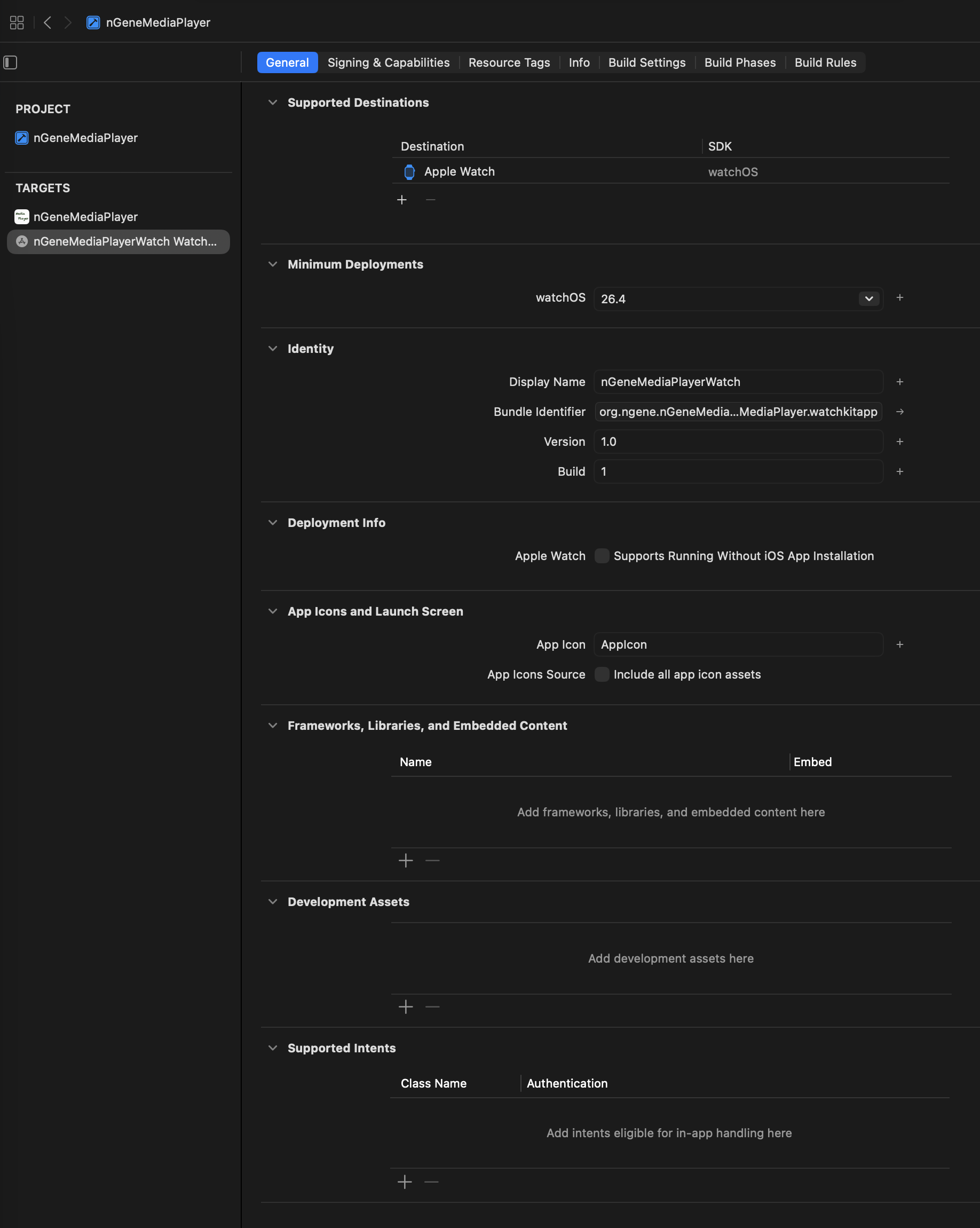
Watch App target general settings
Figure 1. The Watch App target is selected. The Watch App bundle identifier
is visible and ends with .watchkitapp. The
Supports Running Without iOS App Installation checkbox is
not the field that fixes the companion identifier problem.
This screen confirmed that the Watch App target itself had a Watch-style
bundle identifier. That was necessary, but not sufficient. The missing value
was not on this General screen.
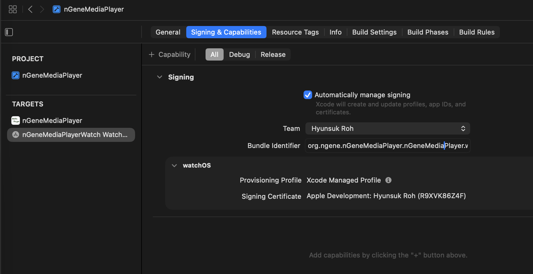
Watch App signing settings
Figure 2. The Watch App Signing & Capabilities tab confirms the Watch
App bundle identifier and signing profile. This still does not fill in
WKCompanionAppBundleIdentifier.
Signing can be valid while installation still fails. In this case, signing was
not the main issue. The generated Info.plist value for the companion app was
the missing part.
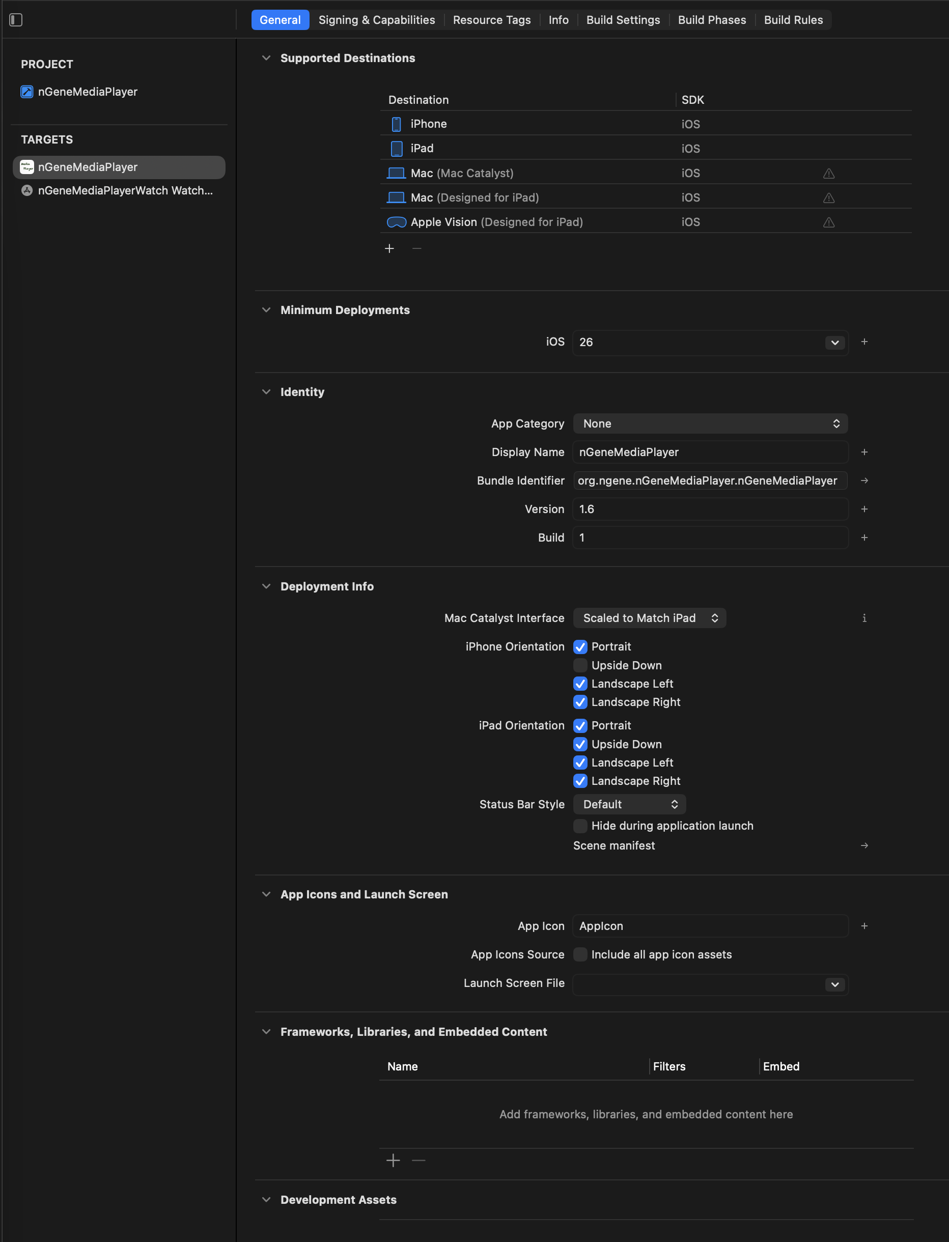
iOS app target bundle identifier
Figure 3. The iOS app target shows the companion value that must be copied:
org.ngene.nGeneMediaPlayer.nGeneMediaPlayer.
This screen provided the correct value for the companion identifier. The
Watch App should point to this exact iOS bundle identifier.
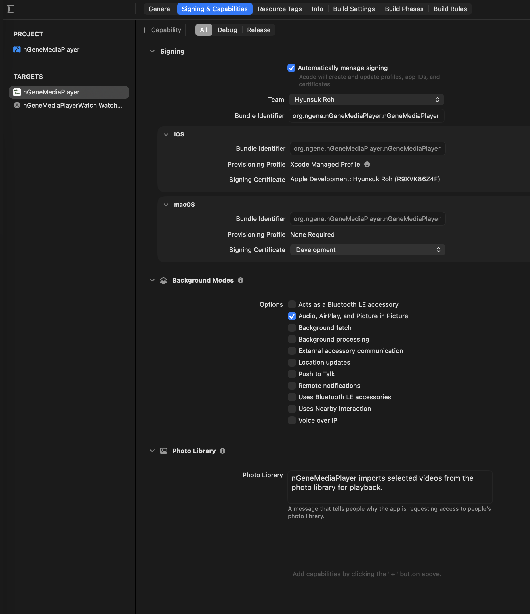
iOS app signing settings
Figure 4. The iOS Signing & Capabilities tab confirms the same iOS app
bundle identifier. This value is the value that belongs in the Watch App
companion setting.
The same iOS bundle identifier appeared in both the General and Signing
screens. That made the correct companion value clear.
Potential confusion between project settings and target settings
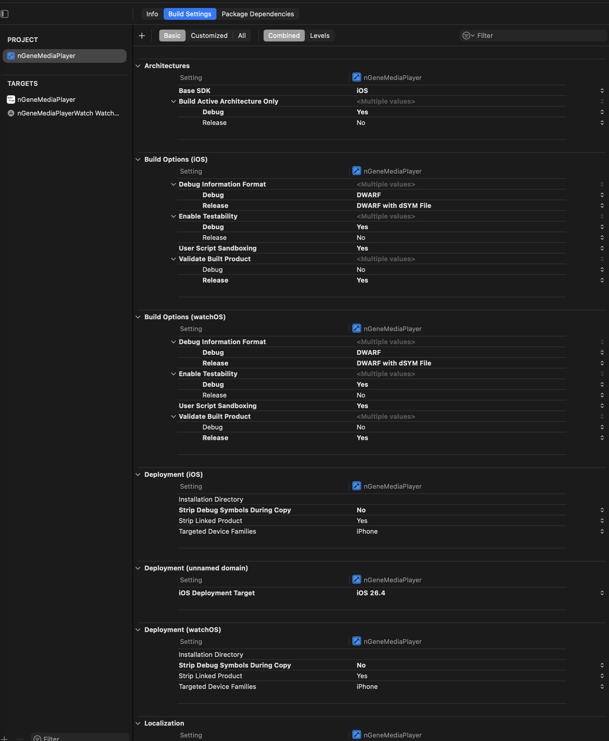
Figure 5. This screen can be misleading because the project itself is
selected. For this issue, the Watch App target must be selected before
editing the Info.plist value.
Editing a project-level setting may not place the value into the generated
Info.plist for the Watch App target. The target column and selected item on
the left side must be checked carefully.
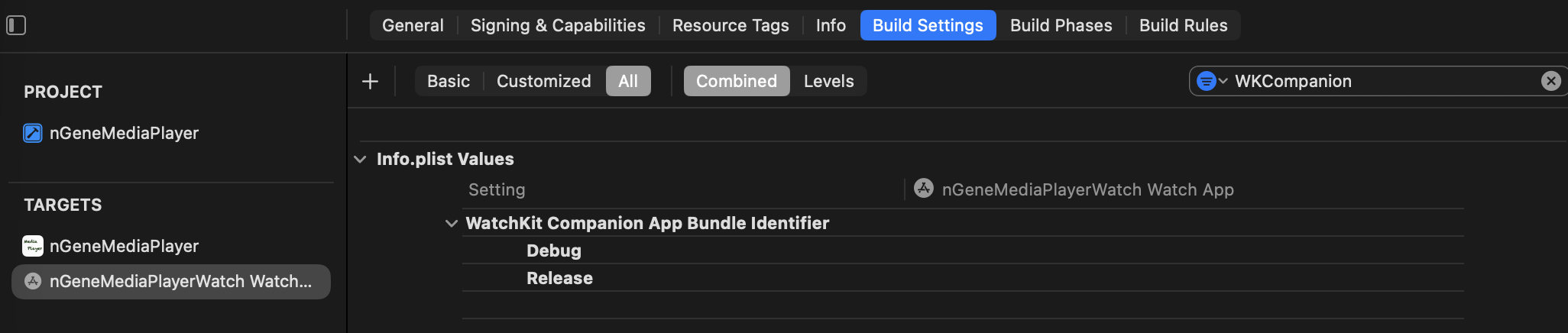
The actual empty setting
Figure 6. This was the decisive screen. The Watch App target is selected,
and the WatchKit Companion App Bundle Identifier setting
is visible, but the Debug and Release values are empty.
The value org.ngene.nGeneMediaPlayer.nGeneMediaPlayer belongs in
the blank value cells for both Debug and Release.
V. The exact fix
Select the correct target
In the Xcode project editor, the selected item on the left side must be:
TARGETS > nGeneMediaPlayerWatch Watch App
The selected item must not be:
PROJECT > nGeneMediaPlayer
Open the correct Build Settings view
Open:
Build Settings > All > Combined
Search for:
WKCompanion
Enter the value in both Debug and Release
Under WatchKit Companion App Bundle Identifier, double-click
the blank cell on the Debug row and enter:
org.ngene.nGeneMediaPlayer.nGeneMediaPlayer
Then double-click the blank cell on the Release row and enter the same value:
This identifies the iOS app paired with the Watch App.
Supports Running Without iOS App Installation
Unchecked
The Watch App is a companion remote, not a standalone watch-only app.
Debug and Release values
Both filled
The simulator may install Debug builds, while archive and distribution use Release.
VII. Clean rebuild procedure after the fix
Clean the build folder
Run:
Product > Clean Build Folder
Remove stale simulator installations
Delete the old Watch App from the Watch simulator and, if needed, delete the
iOS app from the paired iPhone simulator. This avoids confusion from stale
installed bundles.
Run in a stable order
Run the iOS app first on the iPhone simulator. Then run the Watch App on the
paired Watch simulator. This sequence makes the companion relationship easier
to validate.
Clear Derived Data if the same error remains
If the same installation error appears after the values are filled, remove the
project’s Derived Data folder and build again. Generated Info.plist values can
appear stale after target-setting changes.
VIII. Common mistakes to avoid next time
Do not enter .watchkitapp into
WKCompanionAppBundleIdentifier.
Do not edit only the Project-level Build Settings when the Watch App target needs
the value.
Do not rely on the Watch App General tab alone. The Watch App bundle identifier
can be correct while the companion identifier is still empty.
Do not treat Supports Running Without iOS App Installation as the
solution for a companion remote-control Watch App.
Do not assume signing success means installation success. Signing and companion
validation are separate checks.
If an unexpected app name appears in the installation error, check the active
scheme, selected run destination, product name, and whether a Watch target was
copied from another iOS app.
IX. Compact next-time response
When a Watch App installation fails with
InvalidCompanionAppBundleIdentifier, first select the Watch App target,
open Build Settings > All > Combined, search
WKCompanion, and fill both Debug and Release with the iOS app bundle
identifier. The value should not include .watchkitapp.
Watch app companion identifier troubleshooting 한국어 버전
I. 요약
이번 설치 실패의 원인은 Watch App 자체의 bundle identifier가 아니라,
Watch App이 어느 iOS app의 companion인지 알려주는 값이 비어 있었기 때문입니다.
이 Watch App은 watch-only app이 아니라 iOS media player를 조작하는
paired remote-control app입니다. 따라서 generated Watch App Info.plist 안에
유효한 WKCompanionAppBundleIdentifier가 들어가야 합니다.
가장 중요한 구분:
Watch App bundle identifier와 companion iOS app bundle identifier는 서로 다른
필드입니다. Watch App bundle identifier는 보통 .watchkitapp으로
끝납니다. 그러나 companion identifier에는 .watchkitapp을 붙이지
않고 iOS app bundle identifier를 그대로 넣어야 합니다.
II. 에러 메시지의 의미
관찰된 설치 실패
설치 메시지는 app이 WKWatchOnly = TRUE로 watch-only app임을
선언하지 않았다고 말했습니다. watch-only가 아니라면 watchOS는 이 Watch
App이 어느 iOS app에 속하는지 알아야 합니다.
그 관계를 알려주는 generated Info.plist key가 아래입니다.
WKCompanionAppBundleIdentifier
이번 실패는 이 값이 비어 있거나 올바르지 않았기 때문에 발생했습니다.
이 project에서 문제가 생긴 이유
Watch App target은 생성되었고 Watch App 자체의 bundle identifier도
보였습니다. 그러나 companion key가 Build Settings에서 아직 비어
있었습니다. 그래서 build는 되었지만, Watch simulator에 설치되는
단계에서 watchOS가 pairing 관계를 검증하지 못했습니다.
watch-only로 설정하는 것이 올바른 해결책이 아닌 이유
이 Watch App은 iPhone app의 remote control입니다. playback, waveform
state, volume, seeking, A/B loop control의 source of truth는 iOS app에
있습니다. 따라서 WKWatchOnly = TRUE로 설정하면 app의 실제
구조와 맞지 않는 설명이 됩니다.
실무 규칙:
Watch App의 PRODUCT_BUNDLE_IDENTIFIER는
.watchkitapp으로 끝날 수 있습니다. 그러나
WKCompanionAppBundleIdentifier는 iOS app bundle identifier를
가리켜야 하며, .watchkitapp으로 끝나면 안 됩니다.
IV. Screenshot 기준 진단
Watch App target의 General 설정
Figure 1. Watch App target이 선택되어 있습니다. Watch App bundle
identifier가 보이고 .watchkitapp으로 끝납니다.
Supports Running Without iOS App Installation checkbox는
companion identifier 문제를 고치는 필드가 아닙니다.
이 화면은 Watch App target 자체의 bundle identifier가 Watch-style로
설정되어 있음을 확인해 줍니다. 그러나 이것만으로는 충분하지 않습니다.
누락된 값은 이 General 화면에 있지 않았습니다.
Signing이 정상이어도 installation이 실패할 수 있습니다. 이번 경우에는
signing 자체가 핵심 문제가 아니었습니다. generated Info.plist에 들어갈
companion app 값이 빠져 있던 것이 문제였습니다.
iOS app target bundle identifier
Figure 3. iOS app target에는 companion value로 복사해야 할 값이
보입니다. 이 값은
org.ngene.nGeneMediaPlayer.nGeneMediaPlayer입니다.
이 화면이 companion identifier에 넣어야 할 정확한 값을 제공합니다.
Watch App은 이 iOS bundle identifier를 가리켜야 합니다.
iOS app signing 설정
Figure 4. iOS Signing & Capabilities tab에서도 같은 iOS app bundle
identifier가 확인됩니다. 이 값이 Watch App companion setting에
들어가야 합니다.
같은 iOS bundle identifier가 General 화면과 Signing 화면에 모두
나타났습니다. 따라서 companion value로 사용할 값이 명확해졌습니다.
Project settings와 target settings의 혼동 가능성
Figure 5. 이 화면은 project 자체가 선택되어 있어 혼동을 만들 수
있습니다. 이번 문제에서는 Watch App target을 선택한 상태에서
Info.plist value를 수정해야 합니다.
Project-level setting을 수정해도 Watch App target의 generated Info.plist에
값이 들어가지 않을 수 있습니다. 왼쪽에서 어떤 항목이 선택되어 있는지,
그리고 오른쪽 표의 target column이 무엇인지 주의 깊게 확인해야 합니다.
실제로 비어 있었던 setting
Figure 6. 결정적인 화면입니다. Watch App target이 선택되어 있고,
WatchKit Companion App Bundle Identifier setting이
보이지만 Debug와 Release 값이 비어 있습니다.
org.ngene.nGeneMediaPlayer.nGeneMediaPlayer는 Debug와 Release의
빈 value cell에 모두 들어가야 합니다.
V. 정확한 해결 방법
올바른 target 선택
Xcode project editor에서 왼쪽 선택 항목은 반드시 아래여야 합니다.
TARGETS > nGeneMediaPlayerWatch Watch App
아래가 선택된 상태에서 고치면 안 됩니다.
PROJECT > nGeneMediaPlayer
올바른 Build Settings 화면 열기
다음 화면을 엽니다.
Build Settings > All > Combined
검색창에는 아래를 입력합니다.
WKCompanion
Debug와 Release에 모두 값 입력
WatchKit Companion App Bundle Identifier 아래에서 Debug row의
빈칸을 더블클릭하고 아래 값을 입력합니다.
Banksy exhibition photography and copyright use in nGeneColorCube (Written July 23, 2026)
This document analyses photographs taken at a Banksy exhibition from the perspectives of copyright,
exhibition conditions, software distribution, online publication, moral rights, photography rights,
trademark and endorsement risk, and the potentially overlapping rights associated with the five
exhibition categories shown in the guide.
The displayed guide classifies the exhibits as
PCO,
POW,
PHOTO ARCHIVE,
PROJECT ARCHIVE,
and
WCP.
These labels describe provenance, production history, or curatorial classification. They do not, by
themselves, grant visitors permission to photograph, reproduce, publish, distribute, or commercially
exploit the exhibited material.
Core conclusion.
The category guide in the photograph is not a photography-permission notice. Whether a photograph may
be taken must be determined from a separate venue notice, ticket condition, staff instruction, or
work-specific sign. Even where personal photography is permitted, that permission ordinarily covers
the act of taking a personal photograph only. It does not automatically authorise inclusion of the
photograph in a free or paid app, an App Store listing, a product homepage, an advertisement, or a
downloadable online gallery.
I. Four answers at a glance
CHECK FIRST
May a photograph be taken?
Only where the separate venue or work-specific photography rules permit it. The five-category
sign does not answer that question.
GENERALLY LOWER RISK
May the photograph be analysed privately?
Private, local analysis on the same device is generally the lowest-risk use, particularly where
the source file is not uploaded, retained, or publicly displayed.
WRITTEN PERMISSION
May it be included in free or paid software?
Not safely without an express licence. Free software is still publicly distributed software and
may still involve product promotion, user acquisition, advertising, data collection, or future
monetisation.
CONTEXT DEPENDENT
May it be posted on a blog or homepage?
A limited image used as evidence in a genuine review may be arguable. Decorative, promotional,
high-resolution, monetised, or product-marketing use normally requires permission.
Decision key:Generally lower riskConditionalPermission requiredMultiple rights layers
II. Visual guide to the five exhibition categories
PCO
Authentication and original works
Memory cue: authenticity is not a reproduction licence.
POW
Officially released prints and editions
Memory cue: an authorised edition is not an open digital asset.
PHOTO ARCHIVE
Professional photographs of Banksy murals
Memory cue: the photograph and the depicted artwork may both be protected.
PROJECT ARCHIVE
Objects and printed materials from official projects
Memory cue: several creators, producers, and project rights may overlap.
WCP
Reconstructed or restored print archive
Memory cue: reconstruction does not place the underlying image in the public domain.
III. Core legal framework
The category guide is not a photography licence
The photographed sign explains the provenance and character of the exhibits. It does not state
whether photography is allowed, whether only personal photography is allowed, or whether publication
and commercial use are allowed.
Photography permission must therefore be checked separately through the ticket terms, entrance
notice, room-specific sign, staff instruction, or work-specific label. A more restrictive notice
beside a particular photograph, video, object, or installation should prevail over a general
photography policy.
Copyright normally arises automatically
Copyright in an original painting, drawing, stencil, print, photograph, graphic design, or written
work normally arises when the work is created and fixed in a perceptible form. Registration,
publication of the creator’s legal name, a PCO certificate, or the owner’s consent to exhibition
is not what creates the copyright.
Banksy’s phrase “copyright is for losers” is not a reliable worldwide abandonment of
copyright. A provocative statement about copyright does not ordinarily constitute a precise,
irrevocable, worldwide licence permitting all third parties to reproduce and commercially exploit
every work.
A mural created without the property owner’s permission is not automatically copyright-free.
Ownership of the wall, liability for painting the wall, the right to remove the paint, and
copyright in the visual expression are separate legal issues.
Anonymity does not ordinarily eliminate copyright
Copyright systems recognise anonymous and pseudonymous works. Anonymity may make it more difficult
to prove authorship, ownership, assignment, authority to sue, or the authority of an intermediary,
but it does not ordinarily prevent copyright from arising.
The identity described in the 2026 investigative reporting remains distinct from an admission by
the artist or a judicial determination of authorship. Even if the reported identity were later
conclusively established, copyright would not suddenly be “recovered.” The rights would already
have existed; identification could merely make authorship and enforcement easier to prove.
The opposite conclusion is equally important: the absence of a confirmed legal identity does not
place recent Banksy works in the public domain.
The trademark cases did not abolish copyright
The disputes concerning Banksy-related signs and images were trademark proceedings. Some
registrations were initially invalidated on grounds including bad faith and lack of genuine
commercial intention, while a later appeal reversed the cancellation of at least one mark.
Those decisions did not establish that anonymous artists cannot own copyright. Nor did they grant
the public a general right to reproduce Banksy images. Trademark validity, copyright ownership,
moral rights, passing off, false endorsement, and unfair competition remain separate questions.
Incorrect shortcut:
“A Banksy trademark was cancelled, therefore the artwork is copyright-free.”
Correct approach:
Trademark and copyright must be analysed independently for the precise image and proposed use.
Five separate rights gates must be cleared
GATE 1
Venue permission
May the photograph be taken?
→
GATE 2
Underlying artwork
Who controls the Banksy image?
→
GATE 3
Additional layers
Photographer, printmaker, designer, producer.
→
GATE 4
Publication and distribution
App, server, website, social media, advertising.
→
GATE 5
Brand and personal rights
Endorsement, trademarks, visitors, privacy.
Permission at one gate does not clear the others. A venue may permit the camera shutter to be
pressed without owning the right to license the underlying image for software distribution. A
collector may own a PCO-certified print without owning its copyright. A photographer may permit
use of a photograph without having authority to license the artwork appearing inside it.
Ownership of the visitor photograph is only one layer
A visitor may own copyright in original photographic choices such as composition, angle,
perspective, timing, and lighting. That copyright covers the visitor’s new photographic expression.
It does not erase or replace the rights in the Banksy artwork, an archive photograph, a project
design, an edition, or other protected content reproduced inside the photograph.
Practical formula:
owning the photograph file does not necessarily mean owning every right visible inside that file.
IV. May photographs be taken inside the exhibition?
The separate venue rule controls the initial act of photography
Where the venue expressly allows ordinary personal photography, a handheld photograph for a
private camera roll will generally present lower contractual risk. Flash, tripod, selfie-stick,
video, professional equipment, or work-specific restrictions must still be respected where
stated.
Where the venue prohibits commercial-purpose photography, a photograph planned from the outset
for a paid app, product campaign, sponsored article, stock-image library, App Store listing, or
business website may breach the admission conditions even before copyright publication issues
are considered.
Taking a photograph and publishing it are different acts
A personal photograph stored privately is materially different from uploading the file to a
website, embedding it in an executable app, keeping it on a public server, distributing it in a
tutorial, or using it in advertising.
Personal photography permission should therefore be interpreted narrowly unless the venue has
expressly granted broader reproduction and commercial-publication rights in writing.
Private copying does not normally cover public software distribution
Copyright law may provide a limited exception for reproduction made for personal, family-like,
or similarly confined non-commercial use. Once the same file is supplied to an indefinite number
of app users, displayed on a public webpage, or transmitted through a server, the use is no longer
confined to a private circle.
The permanent-public-display exception is unlikely to govern an indoor temporary exhibition
Rules concerning works permanently displayed on streets, in parks, or on building exteriors
should not be assumed to apply to an indoor, admission-controlled, temporary exhibition.
The fact that an original mural may once have appeared outdoors does not automatically free an
indoor print, photograph, reconstruction, restoration, or archive display. The precise exhibited
object must be analysed.
Incidental background inclusion is different from reproducing the work itself
A work appearing incidentally and at small scale in a broader photograph of an exhibition room
may be assessed more favourably than a straight-on photograph in which the work fills most of
the frame. A centred, high-resolution image intended to preserve the work is difficult to
characterise as incidental.
Visitors and exhibition design create additional concerns
Identifiable visitors should be removed, cropped, or obscured before public or commercial use.
Captions, room graphics, video projections, sound, lighting, typography, and exhibition design
may also contain separately protected material.
V. Application to nGeneColorCube
The safest and riskiest software architectures are visually distinct
SAFER STRUCTURE
User-selected image
↓
Local processing on the device
↓
Non-reconstructive palette or colour statistics
↓
No permanent source-image retention
HIGH-RISK STRUCTURE
Developer-selected Banksy photograph
↓
Bundled in the app or stored on a server
↓
Displayed in onboarding or screenshots
↓
Used to promote public software
The legal distinction does not depend only on the image-processing algorithm. It also depends on
who selected the image, who reproduced it, whether it was uploaded or retained, whether it was
publicly displayed, and whether it was used to promote the product.
Free software is not equivalent to private use
A free app can still involve public distribution, brand promotion, user acquisition, advertising,
donations, data collection, investor presentation, commercial goodwill, or future monetisation.
Even a genuinely free and advertisement-free app is distributed beyond a private or family-like
circle.
The absence of a purchase price may reduce one adverse fair-use factor, but it does not create a
copyright licence.
Aggregate colour data is safer than a recognisable source image
Lower-risk output
RGB or Lab values, frequency tables, dominant-colour percentages, a short palette, or a
non-spatial colour cloud that cannot reconstruct the original composition.
Conditional output
A small thumbnail used only while the individual analyses a locally stored image and not
retained, published, or reused by the operator.
Higher-risk output
A full image, recognisable crop, pixel-position map, before-and-after display, or output
capable of reconstructing the source composition.
Individual colours and bare measurements ordinarily contain less protectable expression than the
work’s figures, text, arrangement, and composition. The risk rises where spatial relationships
are retained or the result remains recognisably derived from the work.
Recolouring, distortion, removal of a signature, compositing, or other alteration may also add
attribution and integrity-right concerns.
Software-use matrix
nGeneColorCube scenario
Visual status
Assessment
Recommended control
Private analysis on the same device
Lower risk
The strongest personal-use scenario, provided that the photograph was lawfully
taken and is not publicly transmitted.
Use local processing and avoid automatic upload, public sharing, and permanent
retention.
Unpublished internal development test
Conditional
Practical exposure is limited, but the asset should not remain in a public
repository, release build, tutorial, or marketing capture.
Mark the asset as test-only and remove every copy before release.
Only non-spatial aggregate colour data is retained
Lower risk
Risk is reduced where the original composition cannot be reconstructed and no
source thumbnail is displayed.
Delete the source after local processing and prevent reconstruction from stored
output.
A free app bundles the photograph as a default sample
Permission required
Public reproduction and distribution occur even where no purchase price is
charged.
Replace the photograph or obtain an express written software-distribution
licence.
A paid, subscription, advertising-supported, or in-app-purchase version bundles it
Very high risk
This is direct commercial exploitation and may also conflict with venue
restrictions on commercial-purpose photography.
Do not use without a clearly documented commercial licence.
App Store screenshots, preview video, onboarding, website, or press kit
Very high risk
These are promotional uses even where the app itself is free.
Use owned, commissioned, public-domain, or expressly licensed demo material.
User photographs are uploaded to a private analysis server
Conditional
Server reproduction, storage, security, and privacy exposure arise even where
the user selected the material.
Minimise retention, prohibit unlawful uploads, secure the files, and maintain an
effective complaint-and-removal process.
The app provides a public gallery or sharing feed
High risk
The service facilitates public transmission and may receive infringement,
privacy, and endorsement complaints.
Avoid a default public gallery or implement moderation, reporting, prompt
removal, and repeat-infringer controls.
App branding must not imply Banksy endorsement
Banksy’s name, signature, images, distinctive signs, or PCO terminology should not be used in the
app title, icon, subtitle, keyword strategy, promotional copy, or advertising in a manner that
suggests sponsorship, collaboration, certification, or endorsement.
A disclaimer may be useful, but it does not necessarily cure an overall commercial presentation
that is misleading.
VI. Blog and homepage publication
A genuine review is stronger than decorative publication
Stronger review structure
Substantial original criticism + a small number of necessary images + reduced resolution
+ a direct connection between each image and the analysis + no download function.
Copyright exceptions for quotation, criticism, reporting, education, or fair use depend on the
purpose, character, amount, necessity, proportionality, and market effect of the use. The
photograph should function as evidence supporting the article rather than as the principal
attraction or an online substitute for the exhibition.
Publication matrix
Publication form
Visual status
Practical conclusion
Personal, advertisement-free exhibition diary
Conditional
Use only a small number of necessary, reduced-resolution photographs and add
substantial original commentary.
Critical or educational article analysing the displayed work
Conditional
Each image should be linked to a specific analytical passage and limited to what
is reasonably necessary.
One or two casual personal social-media photographs
Lower practical exposure
Public posting remains outside purely private use. Avoid full galleries,
high-resolution files, promotional wording, and misleading endorsement.
Monetised blog with advertising, sponsorship, or affiliate links
High risk
Commerciality weighs against an exception, particularly where the images attract
traffic or supply the page’s principal value.
nGeneColorCube product homepage, launch article, or feature demonstration
Permission required
This is software promotion. Adding descriptive text does not automatically
transform the use into criticism.
Full exhibition gallery, wallpaper, archive, or downloadable photograph
Do not publish without permission
Such use can substitute for authorised viewing or reproduction and normally
exceeds what is needed for a review.
Minimum safeguards for a review article
The article and analysis should be the principal work, not the image collection.
Each photograph should support a specific passage of criticism, reporting, or education.
Only the number of images reasonably necessary for that purpose should be used.
Reduced-resolution images should be preferred over files suitable for printing or reuse.
Artist, work title, photographer, exhibition, and source should be acknowledged where known.
No download button, wallpaper, merchandise, template, or source-image API should be provided.
No wording should imply endorsement by Banksy, PCO, the photographer, or the organiser.
Attribution should not be treated as a substitute for permission or a valid statutory exception.
VII. Rights-coverage map for PCO, POW, PHOTO ARCHIVE, PROJECT ARCHIVE, and WCP
The following map shows which rights layers are most likely to require attention. It is a visual
screening tool rather than a statement that every possible right necessarily exists in every individual
exhibit.
Primary layerPossible additional layerSecondary or context-dependent
Category
Banksy artwork
Photography rights
Edition, print, or reconstruction
Project, design, or contributor rights
Venue and contract
Commercial-clearance burden
PCO
Primary
Possible
Context-dependent
Possible
Primary
High
POW
Primary
Possible
Primary
Possible
Primary
High
PHOTO ARCHIVE
Primary
Primary
Context-dependent
Possible
Primary
Very high
PROJECT ARCHIVE
Primary
Possible
Possible
Primary
Primary
Very high
WCP
Primary
Possible
Primary
Possible
Primary
Very high
VIII. Category-by-category legal analysis
Category
Meaning and legal significance
Personal photography
Review blog
Free software
Paid or promotional software
Key legal warning
PCO
Pest Control Office
Original works verified by PCO and commonly accompanied by a Certificate of Authenticity.
The certificate concerns authenticity and provenance.
Conditional
Permissible only where the separate venue rule permits personal photography and no
work-specific prohibition applies.
Limited review use
A reduced image may be arguable where directly necessary for criticism or reporting.
Permission required
Do not use without licence
Authentication is not copyright permission. Ownership of a PCO-certified
original does not transfer software, website, advertising, or public-transmission rights.
POW
Pictures on Walls
Prints and editions officially produced and distributed through Pictures on Walls during
the period stated in the exhibition guide.
Conditional
Subject to the separate venue policy and any restriction attached to the particular
edition.
Limited review use
Permission required
Do not use without licence
Official release is not an open licence. Buying or photographing an
authorised edition does not transfer the underlying reproduction, distribution, or
public-transmission rights.
PHOTO ARCHIVE
Professional photographic records
Photographic records of Banksy murals captured through photographer Kim Woo-il’s
aesthetic lens, as described in the exhibition guide.
Personal capture only
A photograph of the displayed archive photograph may reproduce both the professional
photograph and the Banksy mural depicted inside it.
High caution
Only a narrowly necessary image in a genuine review of the photograph or exhibition
should be considered.
Multiple permissions
Complete rights chain required
Two principal copyright layers may overlap: the photographer’s creative
photograph and the underlying Banksy artwork. Venue permission alone is unlikely to clear
both layers.
PROJECT ARCHIVE
Official-project materials
Original objects and printed materials issued in limited quantities at projects led by
Banksy, as described in the exhibition guide.
Personal capture only
Focused criticism only
Documented rights chain
Project-specific licence
Several contributors may hold rights. Artwork, object design, typography,
photography, text, audiovisual material, music, logos, and producer rights may all be
relevant.
WCP
West Country Prince
A print archive described as reconstructing or restoring the manual silkscreen process
and ink texture associated with early Banksy works.
Personal capture only
High caution
Explicit permission
Complete rights chain required
Reconstruction is not public domain. A purely mechanical reproduction
may have limited new originality, but the underlying Banksy image remains relevant, and
selection, arrangement, photography, printmaking, design, and contractual rights may
still exist.
PCO rule
Certificate = authenticity evidence, not reuse permission.
POW rule
Official edition = lawful edition, not open digital distribution.
Official project = potentially several independent contributors.
WCP rule
Restoration or reconstruction = not a general reuse licence.
IX. Illustrative domain maps
The following charts are visual compliance maps rather than probability calculations or judicial
conclusions. Their purpose is to show why some uses require only a limited review while others require
a complete rights chain.
Category rights-layer and commercial-clearance map
PCOPOWPHOTO ARCHIVEPROJECT ARCHIVEWCP
Deployment-risk map
X. Clearance protocol before publication or release
Create an asset-level rights register
Each proposed image should be recorded with its file name, photographed object, exhibition
category, work title, creator, photographer, source, date of capture, intended use, app screen
or webpage, territories, business model, and evidence of permission.
A general note stating “photography was allowed” is insufficient because photography permission
and republication permission are different.
Clear every relevant rights layer
Depending on the category and proposed use, written permission may be required from:
the exhibition organiser for commercial-purpose photography and use of the exhibition environment;
the owner of the underlying artwork copyright or an authorised representative;
the photographer responsible for PHOTO ARCHIVE material;
the producer, designer, publisher, photographer, writer, or other contributor to PROJECT ARCHIVE material;
the relevant printmaker, archive operator, photographer, and underlying-artwork right holder for WCP material;
identifiable individuals whose appearance is used publicly or commercially.
An organiser can license only the rights it owns or has authority to sublicense.
Define the software and marketing rights precisely
A useful licence should expressly address reproduction, cropping, resizing, colour analysis,
alteration, public transmission, server hosting, executable software, App Store screenshots,
preview videos, websites, social media, press materials, free and paid versions, advertising,
worldwide distribution, duration, updates, platform sublicensing, attribution, and termination.
Do not infer permission from provenance or attribution
The following facts do not independently grant permission:
the exhibit is labelled PCO or POW;
the physical object is genuine or officially released;
the visitor personally took the photograph;
the artist remains anonymous;
a Banksy-related trademark was invalidated;
the artist criticised copyright;
the app is free;
the artist and exhibition are credited.
Use a substitute where clearance cannot be documented
Suitable nGeneColorCube demonstration assets include original abstract colour charts,
independently created photographs, commissioned illustrations accompanied by written rights,
and public-domain or open-licensed images whose licence expressly permits the intended software
and commercial uses.
Apply a release gate
No third-party artwork should enter the production app bundle, public repository, App Store
media, product website, advertisement, press kit, or public tutorial until the rights register
contains either an adequate written licence or a use-specific legal-exception analysis.
XI. Final recommendation
Decision zone
Examples
Recommended decision
Lower-risk zone
Private camera-roll storage, local private analysis, unpublished testing, and
non-reconstructive aggregate colour data.
Generally acceptable with ordinary care
Conditional zone
A small number of reduced-resolution photographs in a genuine, commentary-led,
non-promotional exhibition review.
Use only when necessary and proportionate
Permission-required zone
App bundles, default samples, onboarding, App Store screenshots, business homepages,
advertisements, sponsored posts, downloadable images, and public galleries.
Do not use without an express written licence
Layered-rights red zone
PHOTO ARCHIVE, PROJECT ARCHIVE, and WCP material used in software, advertising, or
commercial online publication.
Complete rights chain required
Recommended nGeneColorCube structure.
Permit users to select their own images, process those images locally, avoid bundling Banksy or
exhibition photographs, delete source files after processing where feasible, and display only
non-reconstructive aggregate colour data. All default samples, screenshots, tutorials, product pages,
and advertising should use independently cleared public-domain, open-licensed, commissioned, or
internally created material.
뱅크시 전시 촬영물과 nGeneColorCube 이용에 관한 저작권 분석
본 문서는 뱅크시 전시에서 촬영한 사진을 저작권, 전시장 이용 조건, 소프트웨어 배포,
온라인 공개, 저작인격권, 사진저작권, 상표 및 보증 관계 오인 위험의 관점에서 분석하고,
안내문에 표시된 다섯 가지 전시 범주별로 중첩될 수 있는 권리를 구체적으로 검토합니다.
사진 속 전시 안내문은 전시물을
PCO,
POW,
PHOTO ARCHIVE,
PROJECT ARCHIVE,
WCP
로 분류하고 있습니다. 이 표시는 작품의 출처, 제작 경위 또는 전시 기획상의 범주를 설명하는
것이며, 관람객에게 촬영·복제·게시·배포·상업적 이용을 허락하는 저작권 라이선스는 아닙니다.
핵심 결론.
사진에 보이는 안내문은 촬영 허용 안내문이 아니라 작품 분류 안내문입니다. 사진을 촬영할 수
있는지는 별도의 전시장 안내, 입장권 약관, 직원 안내 또는 작품별 표지를 확인해야 합니다.
개인 촬영이 허용되더라도 그 허락은 일반적으로 개인 사진을 찍는 행위에 한정됩니다. 촬영물을
무료·유료 앱, 앱스토어 등록 화면, 제품 홈페이지, 광고 또는 다운로드 가능한 온라인 갤러리에
사용하는 권한까지 자동으로 부여하지는 않습니다.
I. 질문에 대한 네 가지 직접 답변
먼저 확인
사진을 찍어도 되는가?
별도의 전시장 또는 작품별 촬영 규칙이 허용하는 경우에만 가능합니다. 다섯 가지 범주를
설명한 안내문만으로는 촬영 허용 여부를 알 수 없습니다.
상대적 저위험
촬영한 사진을 개인적으로 분석해도 되는가?
같은 기기 안에서 비공개로 분석하고, 원본을 업로드·보관·공개하지 않는 구조는 일반적으로
가장 위험이 낮습니다.
서면 허락 필요
무료 또는 유료 소프트웨어에 넣어도 되는가?
명시적인 라이선스 없이는 안전하지 않습니다. 무료 앱도 공중에게 배포되며 제품 홍보,
이용자 확보, 광고, 데이터 수집 또는 향후 수익화와 연결될 수 있습니다.
목적에 따라 판단
블로그 또는 홈페이지에 올려도 되는가?
실제 비평에 필요한 제한적 사진은 검토할 수 있습니다. 장식용, 홍보용, 고해상도,
수익화 또는 제품 마케팅 이용은 원칙적으로 허락이 필요합니다.
판단 표시:상대적 저위험조건부 가능서면 허락 필요다중 권리 중첩
II. 다섯 가지 전시 범주의 시각적 안내
PCO
진품 인증과 오리지널 작품
기억할 원칙: 진품 인증은 복제 허락이 아닙니다.
POW
정식 발매 판화와 에디션
기억할 원칙: 정식 에디션은 무료 디지털 자산이 아닙니다.
PHOTO ARCHIVE
뱅크시 벽화를 기록한 전문 사진
기억할 원칙: 사진과 사진 속 작품이 모두 보호될 수 있습니다.
PROJECT ARCHIVE
공식 프로젝트의 오브제와 인쇄물
기억할 원칙: 여러 창작자와 제작자의 권리가 중첩될 수 있습니다.
WCP
고증·복원 또는 재구성된 판화 아카이브
기억할 원칙: 복원이나 재구성이 원본 이미지를 퍼블릭 도메인으로 만들지는 않습니다.
III. 핵심 법률 구조
작품 분류 안내문은 촬영 허가서가 아닙니다
사진 속 안내문은 전시물의 출처와 성격을 설명합니다. 촬영이 가능한지, 개인 촬영만 가능한지,
촬영한 사진을 공개하거나 상업적으로 사용할 수 있는지는 기재되어 있지 않습니다.
따라서 촬영 허용 여부는 입장권 약관, 입구 안내문, 전시실별 표지, 직원 안내 또는 작품별
표시를 별도로 확인해야 합니다. 특정 사진, 영상, 오브제 또는 설치물 옆에 더 엄격한 제한이
표시되어 있다면 해당 표시가 일반 안내보다 우선합니다.
저작권은 원칙적으로 창작과 동시에 발생합니다
창작성이 있는 회화, 드로잉, 스텐실, 판화, 사진, 그래픽 디자인 및 문구는 일반적으로
작품이 창작되어 인식 가능한 형태로 고정되는 시점에 보호됩니다. 저작권 등록, 작가의
법적 이름 공개, PCO 인증서 또는 전시 소유자의 동의가 저작권을 발생시키는 요건은 아닙니다.
뱅크시의 “copyright is for losers”라는 표현은 전 세계에서 효력이 인정되는
명백한 저작권 포기 선언으로 보기 어렵습니다. 저작권을 비판하는 도발적 표현만으로 제3자가
모든 작품을 무제한 복제하고 상업적으로 이용할 수 있는 정확하고 철회 불가능한 라이선스가
성립하지는 않습니다.
건물 소유자의 동의 없이 벽화가 그려졌더라도 작품이 자동으로 자유 이용물이 되지는 않습니다.
벽의 소유권, 벽화를 그린 행위의 위법성, 도료를 제거할 권리 및 이미지 자체의 저작권은
서로 구분되는 문제입니다.
익명성은 일반적으로 저작권을 소멸시키지 않습니다
저작권 제도는 무명 저작물과 이명 저작물을 보호합니다. 익명성은 저작자, 권리 귀속,
양도 관계, 소송 자격 또는 대리기관의 권한을 입증하기 어렵게 만들 수 있으나, 통상
저작권 자체가 발생하지 않는다는 의미는 아닙니다.
2026년 탐사보도에서 제시된 신원은 작가 본인의 인정 또는 저작자임을 확정한 법원 판결과는
구분됩니다. 향후 보도된 신원이 확정되더라도 저작권이 새롭게 “회복”되는 것은 아닙니다.
권리는 이미 존재하고 있었으며, 신원 확인은 저작자와 권리자의 입증 및 권리 집행을
용이하게 만들 수 있을 뿐입니다.
반대로 공식 신원이 확인되지 않았다는 이유로 최근 뱅크시 작품이 퍼블릭 도메인이 되는 것도
아닙니다.
상표권 사건은 저작권을 없앤 판결이 아닙니다
뱅크시 관련 이미지와 표장에 관한 분쟁은 상표 사건이었습니다. 일부 등록은 악의적 출원이나
진정한 상업적 사용 의사 부족 등을 이유로 처음에 무효가 되었고, 이후 항소 단계에서 일부
무효 결정이 뒤집히기도 하였습니다.
이러한 결정은 익명 예술가가 저작권을 보유할 수 없다는 일반 원칙을 확립하지 않았습니다.
대중에게 뱅크시 이미지를 자유롭게 복제할 수 있는 권한을 부여한 결정도 아닙니다. 상표 등록의
유효성, 저작권, 저작인격권, 출처 혼동, 허위 보증 및 부정경쟁은 각각 별도로 판단해야 합니다.
잘못된 단축 논리:
“뱅크시 관련 상표가 무효가 되었으므로 작품도 저작권이 없다.”
올바른 접근:
구체적인 이미지와 이용 목적에 따라 상표권과 저작권을 각각 독립적으로 검토해야 합니다.
다섯 개의 권리 관문을 각각 통과해야 합니다
관문 1
전시장 허가
사진을 찍을 수 있는가?
→
관문 2
원작 저작권
뱅크시 이미지를 누가 관리하는가?
→
관문 3
추가 권리
사진가, 판화가, 디자이너, 제작자.
→
관문 4
공개와 배포
앱, 서버, 웹사이트, SNS, 광고.
→
관문 5
브랜드와 인격권
보증 관계, 상표, 관람객, 개인정보.
하나의 관문에서 받은 허락이 나머지 관문을 자동으로 통과시켜 주지는 않습니다. 전시장은
카메라 촬영을 허용할 수 있지만, 원작 이미지를 소프트웨어에 배포하도록 허락할 저작권까지
보유하지 않을 수 있습니다. 수집가는 PCO 인증 판화를 소유할 수 있지만 저작권까지 소유하는
것은 아닙니다. 사진작가는 자신의 사진 사용을 허락할 수 있지만 사진 속 원작을 허락할
권한까지 보유하지 않을 수 있습니다.
직접 찍은 사진의 소유권은 하나의 권리 층위에 불과합니다
관람객은 구도, 촬영 각도, 원근, 타이밍 및 조명과 같은 독자적 사진 표현에 관하여
저작권을 보유할 수 있습니다. 그러나 해당 권리는 새롭게 추가된 사진적 표현에 한정됩니다.
사진 속 뱅크시 작품, 전문 아카이브 사진, 프로젝트 디자인, 판화 또는 기타 보호 대상을
소멸시키거나 대체하지는 않습니다.
실무 공식:
사진 파일을 소유한다고 해서 그 파일 안에 보이는 모든 권리를 소유하는 것은 아닙니다.
IV. 전시장 안에서 사진을 찍을 수 있는가
최초 촬영 행위는 별도의 전시장 규칙이 결정합니다
전시장이 일반적인 개인 촬영을 명시적으로 허용한다면 개인 사진첩을 위한 휴대 촬영은
계약상 위험이 상대적으로 낮습니다. 다만 플래시, 삼각대, 셀카봉, 영상, 전문 장비 또는
작품별 제한이 표시되어 있다면 이를 따라야 합니다.
전시장이 상업적 목적의 촬영을 금지한다면, 처음부터 유료 앱, 제품 광고, 협찬 게시물,
스톡 이미지, 앱스토어 등록 화면 또는 사업자 홈페이지에 사용할 의도로 촬영하는 행위는
저작권 공개 문제를 검토하기 전부터 입장 조건에 위반될 수 있습니다.
사진을 찍는 행위와 공개하는 행위는 다릅니다
개인적으로 촬영하여 비공개로 보관하는 행위는 파일을 웹사이트에 올리거나, 실행 가능한
앱에 포함하거나, 공용 서버에 보관하거나, 튜토리얼로 배포하거나, 광고에 사용하는 행위와
법적 성격이 다릅니다.
전시장이 더 넓은 복제 및 상업적 공개 권한을 명시적으로 서면 허락하지 않았다면 개인 촬영
허가는 좁게 해석하는 것이 적절합니다.
사적 복제는 일반적으로 불특정 다수에 대한 앱 배포를 포함하지 않습니다
개인, 가족 또는 이에 준하는 한정된 범위에서 이루어지는 비영리 복제에는 제한적인 예외가
검토될 수 있습니다. 그러나 같은 파일을 불특정 다수의 앱 이용자에게 제공하거나, 공개
웹페이지에 표시하거나, 서버를 통해 전송하면 사적인 범위를 벗어납니다.
공개장소 상시전시 예외는 실내 임시 전시에 적용되기 어렵습니다
거리, 공원 또는 건축물 외벽 등에 항시 전시된 작품에 관한 규정을 실내, 입장 통제 및 기간
한정의 임시 전시에 그대로 적용해서는 안 됩니다.
원래의 벽화가 과거 야외에 존재했다는 이유만으로 실내에 전시된 판화, 사진, 복원물,
재구성물 또는 아카이브 자료가 자유 이용물이 되지는 않습니다. 현재 촬영하는 구체적인
전시물을 기준으로 판단해야 합니다.
배경에 우연히 포함된 경우와 작품 자체를 복제한 경우는 다릅니다
전시장 전체를 촬영하는 과정에서 작품이 작게 우연히 포함된 경우는 작품이 정면에서 화면
대부분을 차지하는 사진보다 유리하게 평가될 수 있습니다. 작품을 보존할 목적으로 촬영한
고해상도 정면 사진은 부수적 포함이라고 보기 어렵습니다.
관람객과 전시 디자인에도 별도의 문제가 생길 수 있습니다
공개 또는 상업적 이용 전에 식별 가능한 관람객은 제외, 크롭 또는 비식별 처리하는 것이
적절합니다. 캡션, 공간 그래픽, 영상 프로젝션, 음향, 조명, 타이포그래피 및 전체 전시
디자인에도 별도의 보호 대상이 존재할 수 있습니다.
V. nGeneColorCube에 대한 구체적 적용
안전한 구조와 위험한 구조는 명확히 구분됩니다
상대적으로 안전한 구조
이용자가 자신의 이미지를 선택
↓
기기 안에서 로컬 처리
↓
원본을 복원할 수 없는 팔레트 또는 색상 통계
↓
원본 이미지를 영구 보관하지 않음
위험이 높은 구조
개발자가 뱅크시 사진을 선택
↓
앱 번들 또는 서버에 저장
↓
온보딩·스크린샷·튜토리얼에 표시
↓
공개 소프트웨어의 홍보 자산으로 사용
법적 차이는 이미지 처리 알고리즘에만 달려 있지 않습니다. 누가 이미지를 선택했는지,
누가 복제했는지, 서버에 업로드하거나 보관했는지, 공중에게 표시했는지 및 제품 홍보에
이용했는지가 함께 중요합니다.
무료 소프트웨어는 사적 이용과 동일하지 않습니다
무료 앱도 공중 배포, 브랜드 홍보, 이용자 확보, 광고, 후원, 데이터 수집, 투자자 설명,
영업상 신용 또는 향후 수익화와 연결될 수 있습니다. 광고가 전혀 없는 완전 무료 앱도
불특정 다수에게 배포되면 개인 또는 가정에 준하는 범위의 이용이 아닙니다.
판매가격이 없다는 사실은 공정이용 판단에서 일부 유리한 요소가 될 수 있지만, 그 자체로
저작권 라이선스를 만들어 내지는 않습니다.
집계 색상 데이터는 식별 가능한 원본 이미지보다 안전합니다
상대적 저위험 출력
RGB·Lab 값, 빈도표, 주요 색상 비율, 짧은 팔레트 또는 원래 구도를 복원할 수 없는
비공간적 색상 클라우드.
조건부 출력
개인이 로컬 이미지 분석 중에만 확인하고 운영자가 저장·공개·재이용하지 않는
작은 썸네일.
고위험 출력
전체 이미지, 식별 가능한 크롭, 픽셀 위치 지도, 전후 비교 화면 또는 원본 구도를
재구성할 수 있는 출력.
개별 색상과 순수 수치 정보는 통상 작품의 인물, 문구, 배열 및 구도보다 보호되는 창작적
표현이 적습니다. 공간적 관계를 보존하거나 결과가 원작을 식별할 수 있을수록 위험이
증가합니다.
식별 가능한 작품의 색을 변경하거나, 왜곡하거나, 서명을 제거하거나, 다른 요소와 합성하면
성명표시권과 동일성유지권 문제가 추가될 수 있습니다.
소프트웨어 이용 형태별 판단표
nGeneColorCube 이용 형태
시각적 판단
법적 평가
권장 통제 방안
같은 기기에서 비공개로 분석
상대적 저위험
사진이 적법하게 촬영되었고 공중송신되지 않는다는 전제에서 가장 강한
사적 이용 사례입니다.
로컬 처리를 사용하고 자동 업로드, 공개 공유 및 영구 보관을 피하는 것이
적절합니다.
외부에 공개되지 않는 내부 개발 테스트
조건부
실무상 노출은 제한적이지만 공개 저장소, 출시 빌드, 튜토리얼 또는 홍보
화면에 남아서는 안 됩니다.
테스트 전용으로 표시하고 출시 전 모든 사본을 제거해야 합니다.
비공간적 집계 색상 데이터만 보관
상대적 저위험
원래 구도를 복원할 수 없고 원본 썸네일을 표시하지 않는다면 위험이
낮아집니다.
로컬 처리 후 원본을 삭제하고 저장 결과로 원본을 복원하지 못하도록 해야
합니다.
무료 앱에 사진을 기본 샘플로 포함
허락 필요
판매가격이 없어도 공중을 상대로 한 복제와 배포가 이루어집니다.
사진을 교체하거나 소프트웨어 배포를 명시적으로 허용하는 서면 라이선스를
받아야 합니다.
유료·구독·광고·인앱결제 버전에 포함
매우 높은 위험
직접적인 상업적 이용이며 전시장에 상업 촬영 제한이 있다면 해당 조건과도
충돌할 수 있습니다.
명확하게 문서화된 상업적 라이선스 없이는 사용하지 않는 것이 타당합니다.
앱스토어 스크린샷·미리보기 영상·온보딩·홈페이지·보도자료
매우 높은 위험
앱이 무료이더라도 제품 홍보를 위한 이용입니다.
자체 제작물, 의뢰 제작물, 퍼블릭 도메인 또는 명시적 이용허락 자산을
사용해야 합니다.
이용자 사진을 비공개 분석 서버에 업로드
조건부
이용자가 이미지를 선택하더라도 서버 복제, 보관, 보안 및 개인정보 위험이
발생합니다.
보관기간을 최소화하고, 위법 업로드를 금지하며, 보안 및 신고·삭제 절차를
마련해야 합니다.
공개 갤러리 또는 공유 피드를 제공
높은 위험
서비스가 공중송신을 가능하게 하며 저작권, 개인정보 및 보증 관계 오인
신고를 받을 수 있습니다.
공개 갤러리를 기본 기능으로 두지 않거나, 심사·신고·신속 삭제·반복
침해자 조치를 갖추어야 합니다.
앱의 명칭과 홍보가 뱅크시의 보증을 암시해서는 안 됩니다
Banksy 명칭, 서명, 대표 이미지, 표장 또는 PCO 용어를 앱 이름, 아이콘, 부제, 검색
키워드, 홍보 문구 또는 광고에 사용하여 후원, 협업, 인증 또는 보증 관계가 있는 것처럼
보이게 해서는 안 됩니다.
면책 문구가 도움이 될 수는 있으나, 전체적인 상업적 표현이 오인을 일으킨다면 단순한
면책 문구만으로 문제가 해결되지 않을 수 있습니다.
VI. 블로그와 홈페이지 공개
실제 비평은 장식적 게시보다 법적 근거가 강합니다
비평성이 강한 구조
충분한 독자적 분석 + 꼭 필요한 소수의 사진 + 저해상도 + 각 사진과 분석 문단의
직접 연결 + 다운로드 기능 없음.
장식성이 강한 구조
고해상도 전체 갤러리 + 짧은 설명 + 방문자 유입 + 제품 홍보 + 광고·협찬 +
원본 다운로드.
인용, 비평, 보도, 교육 또는 공정이용에 관한 예외는 이용 목적과 성격, 사용된 양,
필요성, 비례성 및 시장에 미치는 영향을 종합하여 판단합니다. 사진은 글을 뒷받침하는
증거 역할을 해야 하며, 게시물의 주된 볼거리나 온라인 전시의 대체물이 되어서는 안 됩니다.
공개 형태별 판단표
공개 형태
시각적 판단
실무상 결론
광고가 없는 개인 전시 관람기
조건부
필요한 소수의 저해상도 사진만 사용하고 충분한 독자적 설명을 추가하는
것이 적절합니다.
전시 작품을 분석하는 비평 또는 교육 글
조건부
각 이미지가 구체적인 분석 문단과 연결되고 합리적으로 필요한 범위에
한정되어야 합니다.
개인 소셜미디어에 사진 한두 장 게시
실무상 노출은 비교적 낮음
공개 게시는 순수한 사적 이용의 범위를 벗어납니다. 전체 갤러리,
고해상도 파일, 홍보 문구 및 보증 관계 오인을 피해야 합니다.
광고·협찬·제휴 링크가 있는 수익형 블로그
높은 위험
이미지가 방문자 유입이나 페이지의 주된 가치를 제공할수록 상업성이
예외 인정에 불리하게 작용합니다.
nGeneColorCube 제품 홈페이지·출시 글·기능 시연
허락 필요
소프트웨어 홍보에 해당합니다. 설명 문구를 추가하였다는 이유만으로
비평 목적이 되지는 않습니다.
전시 전체 갤러리·배경화면·아카이브·다운로드 사진
허락 없이 공개하지 않음
허가된 전시 관람이나 복제물의 역할을 대신할 수 있으며 일반적인 후기에
필요한 범위를 초과합니다.
전시 후기에서 적용할 최소 보호조치
이미지 모음이 아니라 글과 분석이 게시물의 중심이어야 합니다.
각 사진은 구체적인 비평, 보도 또는 교육 문단을 뒷받침해야 합니다.
목적에 합리적으로 필요한 수의 사진만 사용해야 합니다.
인쇄나 재사용에 적합한 파일보다 저해상도 이미지를 우선해야 합니다.
알 수 있는 경우 작가, 작품명, 사진작가, 전시 및 출처를 표시해야 합니다.
다운로드 버튼, 배경화면, 상품, 템플릿 또는 원본 이미지 API를 제공하지 않아야 합니다.
뱅크시, PCO, 사진작가 또는 전시 주최자의 보증 관계를 암시해서는 안 됩니다.
출처 표시는 이용허락 또는 적법한 법정 예외를 대신하지 않습니다.
VII. PCO, POW, PHOTO ARCHIVE, PROJECT ARCHIVE 및 WCP 권리 범위 지도
아래 지도는 각 범주에서 특히 확인해야 할 권리 층위를 시각화한 것입니다. 모든 개별 전시물에
표시된 모든 권리가 반드시 존재한다는 의미가 아니라, 공개나 상업 이용 전에 확인해야 할 가능성이
높은 영역을 보여주는 선별 도구입니다.
핵심 권리 층위추가 권리 가능성부수적 또는 사안별 판단
범주
뱅크시 원작
사진저작권
판화·에디션·복원
프로젝트·디자인·기여자 권리
전시장·계약
상업적 권리 정리 부담
PCO
핵심
가능
사안별
가능
핵심
높음
POW
핵심
가능
핵심
가능
핵심
높음
PHOTO ARCHIVE
핵심
핵심
사안별
가능
핵심
매우 높음
PROJECT ARCHIVE
핵심
가능
가능
핵심
핵심
매우 높음
WCP
핵심
가능
핵심
가능
핵심
매우 높음
VIII. 범주별 세부 저작권 분석
범주
의미와 법적 성격
개인 촬영
개인 전시 후기
무료 소프트웨어
유료·홍보용 소프트웨어
핵심 법률 경고
PCO
Pest Control Office
PCO의 검증과 진품 인증서를 받은 오리지널 작품으로 설명되는 범주입니다.
인증서는 진품 여부와 출처에 관한 자료입니다.
조건부
별도의 전시장 규칙이 개인 촬영을 허용하고 작품별 금지 표시가 없는 경우에만
가능합니다.
제한적 후기 이용
비평이나 보도에 직접 필요한 경우 저해상도 이미지를 제한적으로 검토할 수 있습니다.
허락 필요
라이선스 없이는 사용하지 않음
진품 인증은 저작권 이용허락이 아닙니다. PCO 인증 원본을 소유한다고
해서 소프트웨어, 홈페이지, 광고 또는 공중송신 권리가 이전되지는 않습니다.
POW
Pictures on Walls
전시 안내에 표시된 기간 동안 Pictures on Walls를 통하여 정식 제작·유통된 판화와
에디션 작품입니다.
조건부
별도의 전시장 정책과 해당 에디션에 부착된 개별 제한을 따라야 합니다.
제한적 후기 이용
허락 필요
라이선스 없이는 사용하지 않음
정식 발매는 오픈 라이선스가 아닙니다. 정식 에디션을 구매하거나
촬영하더라도 기초 이미지의 복제권, 배포권 및 공중송신권이 이전되지 않습니다.
PHOTO ARCHIVE
전문 사진 기록물
전시 안내상 여러 장소에 남은 뱅크시 벽화를 사진작가 김우일의 미학적 시각으로
기록한 사진 자료입니다.
개인 촬영만
전시된 아카이브 사진을 다시 촬영하면 전문 사진과 그 사진 속 뱅크시 벽화를
동시에 복제할 수 있습니다.
높은 주의
해당 사진 또는 전시를 직접 비평하는 글에서 꼭 필요한 이미지에 한하여
검토하는 것이 적절합니다.
복수의 허락 필요
완전한 권리관계 필요
두 개의 핵심 저작권 층위가 중첩될 수 있습니다. 사진작가의 창작적
사진과 사진 속 뱅크시 원작입니다. 전시 주최자의 허락만으로 두 권리가 모두
정리된다고 보기 어렵습니다.
PROJECT ARCHIVE
공식 프로젝트 자료
전시 안내상 뱅크시가 주도한 공식 프로젝트 현장에서 한정 발매된 오리지널 오브제와
인쇄물입니다.
개인 촬영만
집중된 비평만
문서화된 권리관계 필요
프로젝트별 라이선스 필요
여러 기여자가 권리를 보유할 수 있습니다. 작품, 오브제 디자인,
타이포그래피, 사진, 문구, 영상, 음악, 로고 및 제작자의 권리를 함께 확인해야 합니다.
WCP
West Country Prince
전시 안내상 뱅크시 초기 작품의 수작업 실크스크린 공정과 잉크 질감을 고증·복원하여
구성한 판화 아카이브입니다.
개인 촬영만
높은 주의
명시적 허락 필요
완전한 권리관계 필요
복원은 퍼블릭 도메인을 의미하지 않습니다. 기계적 복제 자체의
새로운 창작성이 제한적일 수는 있으나 기초 뱅크시 이미지는 여전히 문제되며,
선택·배열·사진·판화 제작·디자인 및 계약상 권리가 추가될 수 있습니다.
PCO 원칙
인증서 = 진품 증명이며, 2차 이용허락이 아닙니다.
POW 원칙
정식 에디션 = 적법한 발매이며, 자유로운 디지털 배포가 아닙니다.
PHOTO ARCHIVE 원칙
사진가의 사진 + 사진 속 작품 = 중첩된 권리 정리가 필요합니다.
PROJECT ARCHIVE 원칙
공식 프로젝트 = 여러 독립적인 기여자의 권리가 존재할 수 있습니다.
WCP 원칙
복원·고증·재구성 = 포괄적인 재사용 라이선스가 아닙니다.
IX. 권리 영역을 보여주는 시각적 지도
아래 도표는 분쟁 가능성을 수치로 예측하거나 법원의 결론을 표시하는 자료가 아닙니다. 각 범주의
권리 중첩 정도와 이용 형태별 권리 확인 부담을 직관적으로 이해하기 위한 시각적 지도입니다.
범주별 권리 중첩도와 상업적 권리 정리 지도
PCOPOWPHOTO ARCHIVEPROJECT ARCHIVEWCP
이용 형태별 배포 위험 지도
X. 공개 또는 출시 전 권리 확인 절차
이미지 파일별 권리대장을 작성합니다
각 이미지에 파일명, 촬영 대상, 전시 범주, 작품명, 창작자, 사진작가, 출처, 촬영일,
예정 용도, 사용될 앱 화면 또는 웹페이지, 배포 국가, 사업 모델 및 허락 증빙을 기록하는
것이 적절합니다.
“전시장에서 촬영이 허용되었다”는 일반적 기록만으로는 충분하지 않습니다. 촬영 허가와
재게시 허가는 서로 다르기 때문입니다.
관련된 모든 권리 층위를 정리합니다
범주와 예정 용도에 따라 다음 주체의 서면 허락이 필요할 수 있습니다.
상업적 목적 촬영과 전시 환경 이용에 관한 전시 주최자;
기초 작품의 저작재산권자 또는 적법한 권한을 보유한 대리인;
PHOTO ARCHIVE 자료를 촬영한 사진작가;
PROJECT ARCHIVE의 제작자, 디자이너, 출판자, 사진작가, 작가 및 기타 기여자;
WCP 자료의 판화 제작자, 아카이브 운영자, 사진작가 및 기초 이미지 권리자;
공개 또는 상업적 사진에 식별 가능하게 나타난 사람.
전시 주최자는 자신이 보유하거나 재허락할 권한이 있는 범위만 허락할 수 있습니다.
소프트웨어와 마케팅 이용 범위를 구체적으로 규정합니다
실효성 있는 라이선스에는 복제, 크롭, 크기 변경, 색상 분석, 변형, 공중송신, 서버 호스팅,
실행 가능한 소프트웨어 수록, 앱스토어 스크린샷, 미리보기 영상, 홈페이지, 소셜미디어,
보도자료, 무료·유료 버전, 광고, 전 세계 배포, 이용기간, 업데이트, 플랫폼에 대한 재허락,
출처 표시 및 종료 후 처리 방식이 명시되는 것이 바람직합니다.
출처나 표시만으로 허락을 추정하지 않습니다
다음 사실은 각각 독립적인 이용허락이 아닙니다.
전시물에 PCO 또는 POW 표시가 있다는 사실;
실물 작품이 진품이거나 정식 발매물이라는 사실;
관람객이 사진을 직접 찍었다는 사실;
작가가 익명이라는 사실;
뱅크시 관련 상표가 무효가 된 적이 있다는 사실;
작가가 저작권을 비판했다는 사실;
앱이 무료라는 사실;
작가와 전시의 출처를 표시했다는 사실.
권리관계를 문서화할 수 없다면 대체 이미지를 사용합니다
nGeneColorCube의 적절한 데모 자산에는 직접 만든 추상 색상 차트, 별도로 촬영한 사진,
서면 권리를 확보한 의뢰 일러스트, 그리고 예정된 소프트웨어 및 상업적 이용을 명시적으로
허용하는 퍼블릭 도메인 또는 오픈 라이선스 이미지가 포함될 수 있습니다.
출시 승인 절차를 적용합니다
충분한 서면 라이선스 또는 해당 이용 형태에 맞춘 법적 예외 검토 문서가 권리대장에
존재하기 전에는 제3자 작품을 제작 앱 번들, 공개 저장소, 앱스토어 자료, 제품 홈페이지,
광고, 보도자료 또는 공개 튜토리얼에 포함하지 않는 것이 적절합니다.
XI. 최종 권고
판단 구역
대표 사례
권장 결정
상대적 저위험 구역
개인 사진첩 보관, 기기 내 비공개 분석, 외부에 공개되지 않는 테스트 및 원본을
재구성할 수 없는 집계 색상 데이터.
통상적인 주의를 전제로 대체로 가능
조건부 구역
실제 전시 비평이 중심인 비홍보성 글에서 필요한 저해상도 사진 한두 장을
사용하는 경우.
필요성과 비례성이 인정되는 범위로 제한
허락 필요 구역
앱 번들, 기본 샘플, 온보딩, 앱스토어 스크린샷, 사업자 홈페이지, 광고,
협찬 게시물, 다운로드 이미지 및 공개 갤러리.
명시적 서면 라이선스 없이는 사용하지 않음
권리 중첩 고위험 구역
PHOTO ARCHIVE, PROJECT ARCHIVE 및 WCP 자료를 소프트웨어, 광고 또는 상업적
온라인 게시물에 사용하는 경우.
완전한 권리관계 확인 필요
권장되는 nGeneColorCube 구조.
이용자가 자신의 이미지를 선택하도록 하고, 해당 이미지를 기기 안에서 처리하며, 뱅크시 또는
전시 사진을 앱에 기본 포함하지 않고, 가능한 경우 처리 후 원본을 삭제하며, 원본을 재구성할 수
없는 집계 색상 데이터만 표시하는 구조가 적절합니다. 모든 기본 샘플, 스크린샷, 튜토리얼,
제품 홈페이지 및 광고에는 별도로 권리를 확보한 퍼블릭 도메인, 오픈 라이선스, 의뢰 제작물
또는 자체 제작물을 사용하는 것이 바람직합니다.
Written on July 23, 2026
A photograph is not one permission (Written July 30, 2026)
Art, exhibition, and copyright study note
A photograph is not one permission
Learning to read Banksy exhibition photographs as
layered objects rather than as simple image files
The question behind this note
A venue may allow a photograph to be taken.
That apparently simple permission does not
necessarily explain whether the photograph
may later be published, distributed, altered,
used in advertising, or offered as a
downloadable image.
A more careful starting point
The photograph is better understood as a small
map of overlapping permissions. The camera file
may be new, while several protected works and
contractual conditions remain visible inside it.
The central distinction
Permission to take a photograph
≠
Permission to reproduce and publish the depicted work
≠
Permission to use the image for promotion or commerce
This is a practical study framework rather than a
universal legal conclusion. Copyright exceptions,
moral rights, exhibition contracts, public-display
rules, and fair-use or fair-dealing doctrines differ
by jurisdiction and by the exact facts of each use.
01
The simple question contains several different questions
At first, the issue seems binary: either photography is
allowed or it is not. A closer look suggests that this
frame is too narrow. The permission to press the shutter
is only one stage in a much longer sequence.
Six questions hidden inside one photograph
1
Venue access
What do the ticket terms, entrance signs, room
notices, and staff instructions permit?
2
Camera use
Are ordinary photographs permitted, and are flash,
tripods, video, or commercial-purpose photography
restricted?
3
The new file
Does the photographer contribute original choices
of framing, timing, angle, lighting, or perspective?
4
What is depicted
Does the file reproduce an artwork, archive
photograph, typography, installation, or several
works at once?
5
Later publication
Will the image remain private, or will it enter a
blog, social platform, public gallery, lecture,
software product, or server?
6
Promotion and identity
Could the use suggest endorsement, attract
customers, advertise a product, or expose
identifiable visitors?
Working premise
A sign may explain what an exhibit is without explaining
what may be done with an image of it. Provenance
information and permission information should therefore
be read separately.
02
Why Banksy makes the distinction unusually visible
Banksy’s work brings several tensions into the same frame.
Street visibility, anonymity, anti-establishment language,
authentication, official editions, commercial exhibitions,
and digital circulation can appear to point in opposite
directions. These tensions make the subject interesting,
but they may also encourage legal shortcuts that do not
quite follow.
Five recurring paradoxes
Publicly visible
A work seen in public is not necessarily in the
public domain. Visibility and legal reusability
are different ideas.
Anonymous authorship
Anonymous and pseudonymous works may still receive
copyright protection even when enforcement is
more difficult.
“Copyright is for losers”
A provocative slogan is not normally the same as a
precise, worldwide, and irrevocable reuse licence.
Temporary street work
A mural may disappear, while a high-resolution
digital reproduction can circulate indefinitely.
Authentic object
Proof that an object is genuine does not, by itself,
grant reproduction, publication, or advertising
rights.
These apparent contradictions become easier to understand
once the physical object, underlying artwork, visitor’s
photograph, venue contract, and later publication are
treated as separate layers. The confusion often begins
when one layer is expected to answer a question that
belongs to another.
03
What the five exhibition labels can—and cannot—tell us
The exhibition guide groups items into PCO, POW,
PHOTO ARCHIVE, PROJECT ARCHIVE, and WCP. These labels
are useful because they indicate provenance, production
history, or curatorial context. They should not be
mistaken for photography or republication licences.
Category guide
PCO
Authentication and original works
What it describes
Authenticity, provenance, and works associated
with Pest Control Office certification.
What it does not answer
Whether a visitor may reproduce, publish,
advertise, or distribute an image of the work.
Memory cue
Authenticity is not a reproduction licence.
POW
Official prints and editions
What it describes
Prints or editions released through Pictures
on Walls, as identified by the guide.
What it does not answer
Whether the authorised physical edition is also
an unrestricted digital asset.
Memory cue
Official release is not open digital distribution.
PHOTO ARCHIVE
Photographic records of murals
What it describes
A photographer’s visual record of a Banksy work,
often with its own composition, timing, and
aesthetic choices.
What it does not answer
Whether the photographer’s image and the
underlying artwork have both been cleared.
Memory cue
The photograph and depicted artwork may both matter.
PROJECT ARCHIVE
Objects and materials from projects
What it describes
Printed material, objects, graphics, and related
items connected with official projects.
What it does not answer
Which designers, writers, photographers,
producers, or other contributors may hold
separate rights.
Memory cue
One project may contain several independent creators.
WCP
Reconstructed or restored print material
What it describes
West Country Prince material described by the
guide as reconstructing or restoring print
processes and textures.
What it does not answer
Whether the underlying image, printmaking,
photography, or presentation has been licensed.
Memory cue
Reconstruction does not create a general reuse licence.
Rights-layer comparison
Category
Primary descriptive role
Likely rights layers to examine
Most useful caution
PCO
Authenticity, provenance, and original works
Underlying artwork, venue conditions, and
later publication
A certificate concerns authenticity, not
general reproduction permission.
POW
Official prints and editions
Artwork, edition or print rights, and
venue conditions
An authorised edition remains different
from an open-licensed digital file.
PHOTO ARCHIVE
Professional or curated photographic records
Photographer’s image, depicted artwork,
and venue conditions
At least two major copyright layers may
appear in one display.
PROJECT ARCHIVE
Objects and materials from larger projects
Artwork, design, text, photography,
audiovisual work, and production
Project authorship may be distributed
across several contributors.
WCP
Reconstructed or restored print material
Underlying image, print process,
photography, and presentation
Restoration or reconstruction should not
be confused with public-domain status.
Provenance map, not permission map
None of the five labels, standing alone, answers whether
photography, online publication, software distribution,
advertising, or commercial reuse is permitted.
04
A layered-rights model
The problem becomes more manageable when each permission
is treated as a separate gate. A favourable answer at one
gate does not automatically clear the next.
Six layers that may need separate answers
1
Venue and contract
May the photograph be taken under the
ticket terms and room-specific rules?
2
Underlying artwork
Who controls reproduction and public
communication of the depicted Banksy image?
3
Additional creative works
Is there an archive photograph, graphic
design, text, print, video, music, or
installation?
4
The visitor’s photograph
Which new choices of composition, timing,
angle, or lighting belong to the photographer?
5
Publication and distribution
Will the image remain private or be copied,
uploaded, displayed, or distributed?
6
Identity, endorsement, and privacy
Could the presentation imply sponsorship,
use protected signs, or expose identifiable
visitors?
Practical rule
Permission at one layer does not travel
automatically to the others
A venue may permit camera use without owning every
copyright visible in the room. A collector may own
an authentic object without owning its reproduction
rights. A photographer may own a new photograph
while still depicting protected material.
The organiser can ordinarily grant only those rights that
it owns or has authority to sublicense. A statement such
as “photography permitted” may therefore be meaningful but
limited: it may govern conduct inside the venue without
settling later copyright publication.
05
Common shortcuts that do not fully solve the problem
Several statements sound plausible because each contains
a fragment of truth. The difficulty lies in extending that
fragment farther than it can safely carry.
Shortcut and better question
Shortcut
“Photography was allowed, so the image may
be published anywhere.”
Better question
Did the permission cover only personal capture,
or did it expressly include publication and
commercial reuse?
Shortcut
“The photograph is mine, so everything
visible inside it is mine.”
Better question
Which rights belong to the new photograph,
and which remain attached to the artwork,
archive image, or exhibition material?
Shortcut
“The artist is anonymous, so no copyright exists.”
Better question
How does the relevant law treat anonymous or
pseudonymous works, and who has authority to
administer the rights?
Shortcut
“A trademark dispute made Banksy’s images
copyright-free.”
Better question
What did the trademark decision actually concern,
and what separate copyright question remains?
Shortcut
“The use is free or non-profit, so permission
cannot be required.”
Better question
Is the use still public, promotional,
distributive, or capable of substituting for
an authorised copy?
Shortcut
“Attribution is enough because the artist
has been credited.”
Better question
Is there permission, an applicable legal
exception, and any separate attribution or
integrity obligation?
Physical ownership and copyright ownership remain distinct
Buying an original, authenticated work, or authorised
edition usually transfers the physical object. It does
not necessarily transfer the copyright required to
reproduce the image in publications, advertising,
merchandise, software, or public online galleries.
06
The legal character changes as the image travels
The same photograph may begin as a private memory and
later become a public reproduction, promotional asset,
or commercial product. The pixels may remain unchanged
while the purpose, audience, and legal exposure change.
Image lifecycle
1
Capture
The shutter is pressed under the venue’s admission
and photography conditions.
2
Private storage
The photograph remains in a personal camera roll
or similarly confined setting.
3
Edit or analyse
Cropping, recolouring, compositing, enhancement,
or another transformation is applied.
4
Upload
The file is copied to a server, platform, shared
drive, or public-facing service.
5
Public display
An indefinite audience can view, save, repost,
or capture the image.
6
Promotion or sale
The image supports advertising, branding,
subscriptions, merchandise, traffic, or another
commercial objective.
A practical exposure spectrum
Private and confined
Personal camera roll, private notes, or local
examination without public transmission.
Limited internal use
Unpublished study, closed working material, or
restricted internal review.
Public commentary
Review article, educational presentation, social
post, or public webpage.
Promotional or substitutive
Advertising, product media, merchandise, default
assets, or downloadable galleries.
The absence of a purchase price does not return a public
distribution to the private sphere. A free website or
advertisement-free page can still distribute an image to
an indefinite audience, build a brand, attract traffic,
or create commercial goodwill.
07
One visitor photograph may contain several protected works
A photograph of an exhibition wall may appear to be a
single image. Structurally, it may be closer to a set of
nested frames. This is especially important when the
displayed exhibit is itself a photograph of an artwork.
A photograph inside a photograph
Visitor photograph
Exhibition design and display
Archive photograph
Underlying Banksy artwork
One visible file may preserve
several independent layers of
creative expression
Visitor photograph
Composition, angle, timing, perspective, and
lighting may form a new photographic work.
Exhibition presentation
Labels, typography, graphics, lighting,
arrangement, and room design may have
separate protection.
Archive photograph
The professional photographer may control the
photographic record displayed by the exhibition.
Underlying artwork
The mural, stencil, drawing, text, or print
depicted inside the archive photograph remains
a separate layer.
People and signs
Identifiable visitors, trademarks, captions,
logos, and endorsement implications can add
further concerns.
PHOTO ARCHIVE requires particular care
A visitor’s photograph of a displayed archive photograph
may reproduce both the photographer’s image and the
underlying artwork. Venue permission alone may not answer
either copyright question.
08
Composition changes what the photograph appears to be doing
Composition is not a complete legal test, but it offers a
useful practical clue. A work that appears small and
incidental within a broader documentary photograph raises
a different question from a straight-on, high-resolution
image designed to preserve the work itself.
Three simplified framing patterns
Incidental background
The room, visitors, and exhibition experience
remain the principal subject. The artwork
occupies a minor part of the frame.
Contextual documentation
The work is important, but the frame still
records its scale, installation, room, or
relationship to the exhibition.
Reproduction-like capture
The work fills the frame and surrounding
context is removed. The photograph can
function as a substitute image of the exhibit.
Framing pattern
What the photograph seems to document
Practical signal
Incidental background
A visit, room, crowd, or broader exhibition
environment
The depicted work may be secondary, although
venue and privacy rules still matter.
Contextual documentation
Installation, scale, curatorial arrangement,
or exhibition experience
The relationship between the image and
accompanying commentary becomes important.
Reproduction-like capture
The artwork itself, with little or no
surrounding context
The image is more difficult to describe as
merely incidental or necessary room
documentation.
These examples are visual screening aids rather than
judicial conclusions. Purpose, amount, market effect,
contractual terms, and the law of the relevant
jurisdiction remain important.
09
Reviews and education: the image should support the thought
A genuine review, report, or educational explanation may
present a stronger case than decorative publication. The
distinction does not arise merely because the page contains
text. The image should perform a limited evidentiary role
within substantial original analysis.
Two very different page structures
Commentary-led structure
Question
→
Analysis
→
Necessary image
Substantial criticism or explanation comes
first. A limited, reduced image is used because
a specific visual point cannot be explained as
effectively without it.
Image-led gallery structure
Large image
→
More images
→
Brief caption
High-resolution images supply most of the
page’s value. Commentary is minimal, and the
publication can function as a gallery,
substitute, traffic device, or promotional asset.
Factors that can make a review more defensible
The article remains the principal work rather than
the image collection.
Each photograph supports a particular passage of
criticism, reporting, or education.
The number of images is limited to what the
explanation reasonably requires.
Reduced-resolution images are preferred over files
suitable for printing or reuse.
No download button, wallpaper package, source-image
API, or merchandise file is provided.
Artist, work, photographer, exhibition, and source
information are acknowledged where known.
The layout avoids suggesting sponsorship,
collaboration, certification, or endorsement.
Attribution is not treated as a substitute for
permission or a valid legal exception.
Reduced resolution and commentary are helpful, not magical
No single formatting choice guarantees that an exception
applies. Fair-use, fair-dealing, quotation, criticism,
reporting, and educational exceptions depend on the
jurisdiction and the complete context of the use.
10
Practical use matrix
The following table is not a substitute for legal analysis.
Its purpose is to show how the same photograph can move
from a relatively confined use into a setting where
explicit permission or a complete rights chain becomes
increasingly important.
Use
Practical status
Why the analysis changes
Cautious approach
Private camera-roll storage
Lower practical exposure
The image remains within a confined
personal setting and is not transmitted
to an indefinite audience.
Observe venue rules and avoid automatic
public upload.
Private local study or analysis
Lower practical exposure
The source image remains local and is not
used as a public display or promotional asset.
Minimise retention and avoid outputs that
reconstruct the original composition.
Unpublished internal research note
Conditional
The audience is limited, but copies can
still escape through shared repositories,
presentations, or later publication.
Mark the file as restricted and remove it
before public release.
Closed classroom or professional lecture
Conditional
Educational purpose may be relevant, but
access, necessity, source, amount, and
jurisdiction remain important.
Use only what is needed, restrict access,
and avoid distributing high-resolution copies.
Commentary-led exhibition review
Conditional
The image may support criticism or
reporting, but public reproduction still occurs.
Use few, reduced images directly connected
to substantial analysis.
Casual public social-media post
Conditional
The image has left the private sphere and
can be copied, indexed, reposted, or used
outside its original context.
Avoid full galleries, high-resolution files,
promotional framing, and identifiable visitors.
Monetised blog or sponsored article
Permission ordinarily expected
Images may attract traffic, support
advertising, or become a significant part
of the page’s commercial value.
Obtain permission or use independently
cleared substitute material.
Default image inside public software
Permission ordinarily expected
The image is reproduced and distributed to
an indefinite number of users, even when
the software is free.
Use original, commissioned, public-domain,
or appropriately licensed assets.
Product page, preview, advertisement,
or press kit
Promotional clearance required
The photograph is used to sell, promote,
brand, or attract attention to another offering.
Do not rely on personal-photography
permission or attribution alone.
PHOTO ARCHIVE or PROJECT ARCHIVE used
commercially
Multiple permissions likely
The image may contain an underlying artwork,
photographer’s work, design, text, project
material, and venue restrictions.
Document and clear each relevant layer,
or replace the asset.
Full gallery, wallpaper, merchandise,
or download archive
Avoid without full clearance
The publication can substitute for
authorised reproductions and enable
further uncontrolled reuse.
A complete, use-specific rights chain is
normally necessary.
11
A decision path before public reuse
A short sequence of questions cannot resolve every legal
issue, but it can prevent several common category errors
before an image enters a public article, product,
exhibition, campaign, or archive.
Six-step screening process
1
Was photography actually permitted?
Check the ticket, entrance notice,
room-specific signs, work-specific labels,
and staff instructions.
When photography was prohibited or materially
restricted, later publication should not be used
to bypass that initial problem.
2
What exactly appears in the frame?
Identify original artwork, print, archive
photograph, project material, text, design,
visitors, and trademarks.
A photograph of a photograph or project object
may require more than one rights analysis.
3
What is the precise proposed use?
Private study, review, lecture, social post,
public software, advertisement, merchandise,
and downloadable archives are not equivalent.
Permission should be assessed against the real
deployment, not against a vague label such as
“online use.”
4
Is the image necessary for criticism or explanation?
Consider whether the analytical point could be
made with no image, a smaller crop, lower
resolution, or an original diagram.
Necessity and proportionality are generally more
persuasive than decorative inclusion.
5
Does the use promote, monetise, or imply endorsement?
Consider advertising, subscriptions, product
placement, branding, audience acquisition,
sponsorship, and commercial goodwill.
Promotional presentation usually requires a more
explicit and documented permission basis.
6
Can every relevant permission be documented?
Record the grantor, rights covered, media,
territory, duration, editing permission,
attribution, and commercial scope.
Where the chain remains unclear, an independently
created or clearly licensed substitute is often
the more responsible choice.
12
A modest asset-level rights register
A general note stating that photography was allowed is
rarely detailed enough for later publication. Recording
the intended use for each individual image makes
uncertainty visible before the image is released.
Information worth recording
Field 01
Asset identity
File name, capture date, exhibition, room,
work title, and category.
Field 02
Visible rights layers
Artwork, archive photograph, project design,
text, logo, visitor, or other content.
Field 03
Venue permission
Ticket terms, photography notice, work-specific
restriction, and evidence of staff instructions.
Field 04
Intended use
Review, lecture, public webpage, social post,
software, advertising, press material, or merchandise.
Field 05
Audience and territory
Private, restricted, public, worldwide,
platform-specific, or downloadable.
Field 06
Commercial context
Advertising, subscription, product promotion,
sponsorship, donation, or brand-building role.
Field 07
Permission evidence
Licensor, authority, covered rights, editing
terms, attribution, duration, and termination.
Field 08
Release decision
Approved, restricted, exception analysis required,
replacement needed, or excluded from publication.
Asset
Visible layers
Proposed use
Permission basis
Decision
Exhibition-room photograph
Room design, small background artwork,
and unidentified visitors
Commentary-led exhibition diary
Venue photography rule plus use-specific
review analysis
Use a reduced image only when directly relevant
Straight-on PCO work photograph
Underlying artwork and visitor photograph
Decorative homepage image
No documented reproduction licence
Replace
PHOTO ARCHIVE display photograph
Archive photographer, underlying artwork,
and exhibition presentation
Public promotional material
Incomplete multi-layer clearance
Exclude until every relevant layer is documented
A useful licence may need to address reproduction,
cropping, resizing, colour alteration, public
transmission, server hosting, executable software,
websites, social media, preview media, free and paid
distribution, advertising, territory, duration,
platform sublicensing, attribution, and termination.
The exact list depends on the intended use.
13
What seems most useful after separating the layers
The subject remains fact-sensitive, and a single diagram
cannot settle every dispute. Even so, three distinctions
appear to remove much of the initial confusion.
Three durable principles
1
A category label is descriptive
PCO, POW, PHOTO ARCHIVE, PROJECT ARCHIVE,
and WCP help explain provenance or production
context. They do not automatically function as
public-reuse licences.
2
Owning the file is only one layer
A visitor may create and own a new photograph
while the artwork, archive image, design, text,
and contractual restrictions remain independently
relevant.
3
The proposed use determines the real question
Private storage, criticism, social posting,
public distribution, promotion, and merchandise
should not be treated as variations of the same
permission.
The most useful reframing may be to replace the
question
“Is this photograph mine?”
with
“Which permissions does this particular use require?”
That change does not resolve every case, but it helps
prevent authenticity, physical ownership, camera
permission, copyright, publication, and endorsement
from being collapsed into a single answer.
미술·전시·저작권을 함께 살펴보는 기록
사진 한 장은 하나의 허락이 아니다
뱅크시 전시 사진을 단순한 이미지 파일이 아니라
여러 권리와 조건이 겹쳐 있는 대상으로 차분히 살펴보기
이 글에서 출발한 질문
전시장이 사진 촬영을 허용할 수는 있다.
그러나 그 허락만으로 사진을 나중에 공개하거나,
배포하거나, 수정하거나, 광고에 사용하거나,
내려받을 수 있는 이미지로 제공해도 된다는
결론까지 바로 이어지지는 않는다.
조금 더 조심스러운 출발점
사진은 하나의 파일이라기보다 여러 허락이 겹쳐
있는 작은 지도에 가깝다고 생각해 볼 수 있다.
촬영된 파일은 새로 만들어졌지만, 그 안에는
기존 작품과 계약 조건이 여전히 남아 있을 수 있다.
가장 먼저 구분할 점
사진을 촬영할 수 있다는 허락
≠
사진 속 작품을 복제하고 공개할 수 있다는 허락
≠
사진을 홍보나 상업적 목적으로 사용할 수 있다는 허락
이 글은 모든 상황에 곧바로 적용되는 법률적 결론이라기보다,
복잡한 문제를 하나씩 나누어 살펴보기 위한 실무적 학습
틀에 가깝다. 저작권 제한 규정, 저작인격권, 전시 계약,
공공장소의 작품에 관한 규정, 공정 이용 또는 공정 거래의
범위는 국가와 구체적인 이용 상황에 따라 달라질 수 있다.
01
단순해 보이는 질문 안에는 여러 질문이 들어 있다
처음에는 촬영이 허용되는지 아닌지만 확인하면 될 것처럼
보인다. 그러나 조금 더 들여다보면 이 구분만으로는 충분하지
않다. 셔터를 누르는 행위는 더 긴 이용 과정의 첫 단계일
뿐일 수 있다.
한 장의 사진에 숨어 있는 여섯 가지 질문
1
전시장 이용 조건
입장권 조건, 입구 안내문, 전시실 표지,
직원 안내는 무엇을 허용하고 있는가?
2
카메라 사용
일반 촬영은 허용되는가? 플래시, 삼각대,
동영상, 상업 목적 촬영에는 제한이 있는가?
3
새로 만들어진 파일
구도, 촬영 시점, 각도, 조명, 원근감과 같은
촬영자의 독자적 선택이 포함되어 있는가?
4
사진 안의 대상
작품, 기록 사진, 타이포그래피, 설치물,
또는 여러 창작물이 함께 재현되어 있는가?
5
그 이후의 공개
사진은 개인적으로만 보관되는가, 아니면 블로그,
소셜 플랫폼, 공개 갤러리, 강의, 소프트웨어,
서버에 들어가게 되는가?
6
홍보와 개인 식별
후원이나 협업으로 오해될 수 있는가?
제품을 홍보하거나 방문객의 얼굴을 드러내는가?
이 글의 기본 전제
안내문은 전시물이 무엇인지 설명할 수 있지만,
그 전시물의 사진으로 무엇을 해도 되는지까지 설명하지는
않을 수 있다. 따라서 출처와 진위를 설명하는 정보와,
이용 허락을 설명하는 정보는 구분해서 읽는 편이 타당하다.
02
뱅크시는 이 구분을 유난히 선명하게 보여 준다
뱅크시의 작업에는 서로 반대 방향으로 보이는 요소들이
함께 나타난다. 거리에서 누구나 볼 수 있다는 점, 작가의
익명성, 제도에 대한 비판적 언어, 작품 인증, 공식 에디션,
상업 전시, 디지털 유통이 한 화면 안에서 충돌한다.
이 긴장은 흥미롭지만, 법적 결론을 지나치게 단순화하게
만드는 원인이 되기도 한다.
반복해서 나타나는 다섯 가지 역설
공개적으로 보이는 작품
누구나 볼 수 있다는 사실이 곧바로 공공 영역의
작품이라는 뜻은 아니다. 가시성과 자유로운 재사용은
서로 다른 개념이다.
익명의 저자
익명이나 가명으로 발표된 작품도 보호될 수 있다.
다만 저자와 권리자를 입증하고 권리를 행사하는
과정이 더 어려울 수 있다.
“Copyright is for losers”
도발적인 문장은 모든 작품을 전 세계에서 제한 없이
사용할 수 있도록 허락하는 정확한 라이선스와는
성격이 다르다.
사라질 수 있는 거리 작품
벽화는 훼손되거나 사라질 수 있지만,
고해상도 디지털 복제물은 사실상 무기한
유통될 수 있다.
진품으로 인증된 물건
물건이 진품이라는 사실만으로 복제, 공개,
광고 이용 권한까지 함께 주어지는 것은 아니다.
물리적 작품, 그 작품에 담긴 표현, 방문객이 촬영한 사진,
전시장 계약, 이후의 공개 이용을 서로 다른 층으로 나누어
보면 이러한 모순은 조금 더 이해하기 쉬워진다. 혼란은
한 층의 정보로 다른 층의 질문까지 답하려 할 때 자주
생기는 듯하다.
03
다섯 가지 전시 분류가 알려 주는 것과 알려 주지 않는 것
전시 가이드는 전시물을 PCO, POW, PHOTO ARCHIVE,
PROJECT ARCHIVE, WCP로 나눈다. 이 표시는 작품의 출처,
제작 배경, 전시 맥락을 이해하는 데 유용하다. 다만 그 자체를
촬영 허가나 재공개 허가로 해석하기는 어렵다.
분류별로 살펴보기
PCO
인증과 원작
설명하는 것
Pest Control Office 인증과 관련된 진위,
출처, 원작의 성격을 설명한다.
설명하지 않는 것
방문객이 작품 사진을 복제, 공개, 광고,
배포해도 되는지는 별개의 질문이다.
기억할 문장
진품 인증은 복제 라이선스가 아니다.
POW
공식 판화와 에디션
설명하는 것
가이드에 따르면 Pictures on Walls를 통해
발행된 판화나 에디션을 설명한다.
설명하지 않는 것
공식적으로 발행된 물리적 에디션을 제한 없이
사용할 수 있는 디지털 자산으로 볼 수 있는지는
별개의 문제다.
기억할 문장
공식 발행은 공개 디지털 배포 허락이 아니다.
PHOTO ARCHIVE
벽화를 기록한 사진 작품
설명하는 것
촬영자의 구도, 시점, 빛, 미적 선택이 포함된
뱅크시 작품의 사진 기록을 설명한다.
설명하지 않는 것
사진가의 사진과 그 안에 보이는 원작에 관한
권리가 모두 정리되었는지는 별도로 확인해야 한다.
기억할 문장
사진과 사진 속 작품이 모두 중요할 수 있다.
PROJECT ARCHIVE
프로젝트에서 나온 물건과 인쇄물
설명하는 것
공식 프로젝트와 관련된 인쇄물, 물건,
그래픽, 기타 자료를 설명한다.
설명하지 않는 것
디자이너, 작가, 사진가, 제작자와 같은
여러 기여자 중 누가 어떤 권리를 가지는지는
별도로 살펴보아야 한다.
기억할 문장
하나의 프로젝트에 여러 창작자가 있을 수 있다.
WCP
복원 또는 재현된 판화 자료
설명하는 것
가이드에서 West Country Prince가 판화의
공정과 질감을 복원하거나 재현한 것으로 설명한
자료를 가리킨다.
설명하지 않는 것
원래 이미지, 판화 제작, 사진, 전시 방식의
이용 권리가 모두 허락되었는지는 알 수 없다.
기억할 문장
복원과 재현은 일반적인 재사용 허락이 아니다.
권리 층위 비교
분류
주로 설명하는 내용
함께 살펴볼 가능성이 큰 권리
핵심 주의점
PCO
진위, 출처, 원작
원작의 권리, 전시장 조건, 이후의 공개
인증서는 진위를 설명할 뿐,
일반적인 복제 허락을 의미하지 않는다.
POW
공식 판화와 에디션
원작, 에디션 또는 판화, 전시장 조건
공식 에디션과 공개 라이선스가 적용된
디지털 파일은 서로 다르다.
PHOTO ARCHIVE
전문적 또는 전시용 사진 기록
사진가의 사진, 사진 속 작품, 전시장 조건
한 전시물 안에 적어도 두 개의 주요
저작권 층이 나타날 수 있다.
PROJECT ARCHIVE
더 큰 프로젝트에서 나온 물건과 자료
작품, 디자인, 글, 사진, 영상,
제작 과정
프로젝트의 창작 권리는 여러 기여자에게
나뉘어 있을 수 있다.
WCP
복원 또는 재현된 판화 자료
원래 이미지, 판화 공정, 사진,
전시 표현
복원이나 재현을 공공 영역의 작품과
동일하게 생각해서는 곤란하다.
출처 지도이지, 허락 지도는 아니다
다섯 가지 표시는 그 자체만으로 촬영, 온라인 공개,
소프트웨어 배포, 광고, 상업적 재사용을 허락한다고
말해 주지 않는다.
04
권리를 여러 층으로 나누어 보는 방법
각각의 허락을 별도의 관문으로 생각하면 문제가 조금 더
정리된다. 어느 한 관문에서 긍정적인 답을 얻었다고 해서
그다음 관문까지 자동으로 통과하는 것은 아니다.
별도의 답이 필요할 수 있는 여섯 가지 층
1
전시장과 계약
입장권 조건과 전시실 규칙에 따라
사진을 촬영해도 되는가?
2
사진 속 원작
사진에 보이는 뱅크시 이미지의 복제와
공개를 누가 관리하는가?
3
추가적인 창작물
기록 사진, 그래픽 디자인, 글, 판화,
영상, 음악, 설치물이 함께 있는가?
4
방문객이 촬영한 사진
구도, 시점, 각도, 빛과 같은 새로운
선택 중 무엇이 촬영자의 표현인가?
5
공개와 배포
사진은 개인적으로 남는가, 아니면 복제,
업로드, 전시, 배포되는가?
6
개인 식별·후원 오인·사생활
후원 관계로 오해될 수 있는가?
보호되는 표지나 식별 가능한 방문객이
포함되어 있는가?
실무적으로 기억할 원칙
한 층에서 받은 허락은 다른 층으로
자동 이동하지 않는다
전시장은 카메라 사용을 허락할 수 있지만,
전시장 안에 보이는 모든 저작권을 보유한 것은
아닐 수 있다. 소장자는 진품을 소유하면서도
복제권은 보유하지 않을 수 있다. 촬영자는 새로운
사진에 권리를 가지면서도 보호되는 작품을
사진 안에 담고 있을 수 있다.
전시 주최자는 자신이 보유하거나 다시 허락할 권한이 있는
범위 안에서만 이용을 허락할 수 있다. 따라서
“사진 촬영 가능”이라는 안내는 의미가 있지만 그 범위가
제한적일 수 있다. 전시장 안에서 카메라를 사용하는 행위는
허용하면서도, 이후의 온라인 공개까지 해결해 주지는 않을 수 있다.
05
문제를 완전히 해결하지 못하는 몇 가지 지름길
다음 문장들은 일부 사실을 담고 있어서 그럴듯하게 들린다.
다만 그 일부를 실제로 감당할 수 있는 범위보다 더 멀리
확장하는 순간 문제가 생긴다.
단순화된 결론과 조금 더 나은 질문
단순화된 결론
“촬영이 허용되었으니 어디에든 공개해도 된다.”
조금 더 나은 질문
그 허락은 개인 촬영만을 의미했는가,
아니면 공개와 상업적 재사용까지 명시적으로
포함했는가?
단순화된 결론
“내가 찍은 사진이므로 사진 안의 모든 것도 내 것이다.”
조금 더 나은 질문
새 사진에 관한 권리는 무엇이며,
원작, 기록 사진, 전시 자료에 남아 있는
권리는 무엇인가?
단순화된 결론
“작가가 익명이므로 저작권도 존재하지 않는다.”
조금 더 나은 질문
관련 법은 익명 또는 가명 작품을 어떻게 다루며,
누가 권리를 관리할 권한을 가지고 있는가?
단순화된 결론
“상표권 분쟁이 있었으므로 뱅크시 이미지는
저작권에서도 자유롭다.”
조금 더 나은 질문
해당 판단이 실제로 다룬 것은 무엇이며,
별도로 남아 있는 저작권 문제는 무엇인가?
단순화된 결론
“무료이거나 비영리 목적이면 허락이 필요하지 않다.”
조금 더 나은 질문
무료라 하더라도 공개·홍보·배포 기능을 하거나,
정식 복제물을 대신할 정도의 역할을 하는가?
단순화된 결론
“작가 이름을 밝혔으므로 출처 표기만으로 충분하다.”
조금 더 나은 질문
이용 허락이나 적용 가능한 제한 규정이 있는가?
출처 표시 및 작품의 동일성 유지와 관련된
별도 의무가 있는가?
물리적 소유와 저작권 보유는 구분할 필요가 있다
원작, 인증된 작품, 공식 에디션을 구매하면 대체로
물리적 물건을 소유하게 된다. 그러나 출판물, 광고,
상품, 소프트웨어, 온라인 갤러리에서 이미지를 복제하고
공개할 수 있는 권리까지 반드시 함께 이전되는 것은 아니다.
06
같은 사진도 이동하는 과정에서 이용의 성격이 달라진다
한 장의 사진은 개인적인 기억으로 시작해 공개 복제물,
홍보 자료, 상업적 상품으로 바뀔 수 있다. 픽셀은 동일해도
목적, 이용자 범위, 법적 노출 정도는 크게 달라질 수 있다.
이미지가 이동하는 과정
1
촬영
입장 조건과 촬영 규칙 아래에서 셔터를 누른다.
2
개인 보관
사진이 개인 사진 보관함이나 이와 비슷한
제한된 공간에 머문다.
3
편집 또는 분석
자르기, 색상 변경, 합성, 보정 또는 다른
변형이 적용된다.
4
업로드
파일이 서버, 플랫폼, 공유 저장소,
공개 서비스에 복제된다.
5
공개 전시
불특정한 사람들이 이미지를 보고, 저장하고,
다시 게시하거나 캡처할 수 있게 된다.
6
홍보 또는 판매
사진이 광고, 브랜드, 구독, 상품,
방문자 유입, 다른 상업적 목적을 돕는다.
실무적 노출 범위
개인적이고 제한된 이용
개인 사진 보관함, 비공개 기록,
외부 전송이 없는 로컬 검토.
제한된 내부 이용
공개되지 않은 학습 자료, 내부 작업물,
접근이 제한된 검토.
공개 비평과 설명
전시 리뷰, 교육 발표, 소셜 게시물,
공개 웹페이지.
홍보 또는 대체 이용
광고, 제품 홍보물, 상품, 기본 제공 자산,
내려받을 수 있는 갤러리.
가격을 받지 않는다고 해서 공개 배포가 다시 개인 이용으로
돌아가는 것은 아니다. 무료 웹사이트나 광고가 없는 페이지도
불특정한 사람들에게 이미지를 배포하고, 브랜드를 만들고,
방문자를 모으거나 상업적 신용을 형성할 수 있다.
07
방문객이 촬영한 한 장의 사진 안에 여러 작품이 있을 수 있다
전시 벽을 촬영한 사진은 하나의 이미지처럼 보인다.
그러나 구조적으로는 여러 프레임이 겹쳐 있는 것에 더
가까울 수 있다. 전시물이 작품을 기록한 사진일 때에는
이 점이 특히 중요해진다.
사진 속에 들어 있는 또 다른 사진
방문객이 촬영한 사진
전시 디자인과 배치
기록 사진
사진 속 뱅크시 원작
하나의 파일 안에 독립적인
여러 창작 표현이 함께 남을 수 있다
방문객이 촬영한 사진
구도, 각도, 시점, 원근감, 빛은 새로운
사진 표현을 만들 수 있다.
전시 연출
라벨, 타이포그래피, 그래픽, 조명,
배치, 공간 디자인도 별도의 보호 대상일 수 있다.
기록 사진
전시된 사진 기록에 대해서는 전문 사진가가
권리를 가지고 있을 수 있다.
사진 속 원작
기록 사진에 담긴 벽화, 스텐실, 그림,
글, 판화는 또 하나의 별도 층으로 남는다.
사람과 표지
식별 가능한 방문객, 상표, 캡션, 로고,
후원 관계에 대한 오인 가능성도 더해질 수 있다.
PHOTO ARCHIVE는 특히 조심해서 볼 필요가 있다
전시된 기록 사진을 방문객이 다시 촬영하면,
전문 사진가의 사진과 그 사진 안에 보이는 원작을 모두
재현할 수 있다. 전시장 촬영 허락만으로 이 두 가지
저작권 문제가 모두 해결되지는 않을 수 있다.
08
구도는 사진이 무엇을 하려는 것처럼 보이는지를 바꾼다
구도만으로 법적 결론을 내릴 수는 없다. 다만 실무적으로
유용한 단서는 될 수 있다. 전시실 전체를 기록한 사진의
작은 배경으로 작품이 들어간 경우와, 작품만 정면에서
고해상도로 촬영한 경우는 서로 다른 질문을 만든다.
세 가지 단순화된 촬영 구도
부수적인 배경
전시실, 방문객, 관람 경험이 주된 대상이다.
작품은 화면의 작은 일부만 차지한다.
맥락을 포함한 기록
작품이 중요하지만, 크기, 설치 방식,
전시실, 다른 전시물과의 관계도 함께 기록한다.
복제물에 가까운 촬영
작품이 화면 대부분을 차지하고 주변 맥락은
사라진다. 전시물을 대신하는 이미지처럼
기능할 가능성이 커진다.
구도
사진이 기록하는 것으로 보이는 대상
실무적으로 보이는 신호
부수적인 배경
방문, 전시실, 관람객, 전시 환경 전체
작품의 비중이 작을 수 있지만,
전시장 규칙과 사생활 문제는 여전히 남는다.
맥락을 포함한 기록
설치 방식, 규모, 큐레이션,
관람 경험
사진과 함께 제시되는 설명 및 비평의
관계가 중요해진다.
복제물에 가까운 촬영
주변 맥락이 거의 없는 작품 자체
단순한 배경이나 전시실 기록이라고
설명하기가 더 어려워진다.
이 그림은 사전 검토를 돕기 위한 시각적 도구일 뿐,
법원의 결론을 대신하지 않는다. 이용 목적, 사용된 양,
시장에 미치는 영향, 계약 조건, 관련 국가의 법은
여전히 중요하다.
09
비평과 교육에서는 이미지가 생각을 뒷받침해야 한다
실질적인 비평, 보도, 교육적 설명은 장식적 공개보다
더 설득력 있는 맥락을 가질 수 있다. 그러나 페이지에
글이 있다는 사실만으로 이러한 성격이 생기지는 않는다.
이미지는 충분한 독자적 분석 안에서 제한적인 근거 자료로
기능하는 편이 자연스럽다.
서로 다른 두 가지 페이지 구조
비평과 설명이 중심인 구조
질문
→
분석
→
필요한 이미지
충분한 비평과 설명이 먼저 나온다. 특정한
시각적 논점을 이미지 없이 설명하기 어려울 때,
제한된 크기와 해상도의 이미지를 사용한다.
이미지 갤러리가 중심인 구조
큰 이미지
→
더 많은 이미지
→
짧은 캡션
고해상도 이미지가 페이지 가치의 대부분을
제공하고, 설명은 최소한에 그친다. 이 경우
갤러리, 대체 복제물, 방문자 유입 장치,
홍보 자료처럼 기능할 수 있다.
비평의 성격을 더 분명하게 만드는 요소
이미지 모음이 아니라 글과 분석이 주된 결과물이다.
각 사진이 구체적인 비평, 보도, 교육 문단을
직접 뒷받침한다.
설명에 합리적으로 필요한 수만큼만 이미지를 사용한다.
인쇄나 재사용에 적합한 파일보다 낮은 해상도의
이미지를 우선한다.
다운로드 버튼, 배경화면 묶음, 원본 이미지 API,
상품 제작 파일을 제공하지 않는다.
확인 가능한 범위에서 작가, 작품, 사진가,
전시, 출처를 밝힌다.
후원, 협업, 인증, 공식 추천으로 오해될 수 있는
구성을 피한다.
출처 표시를 이용 허락이나 법률상 제한 규정의
대체물로 생각하지 않는다.
낮은 해상도와 충분한 설명은 도움이 되지만,
자동으로 문제를 해결하지는 않는다
어느 한 가지 편집 방식만으로 제한 규정의 적용이
보장되지는 않는다. 인용, 비평, 보도, 교육,
공정 이용 또는 공정 거래의 범위는 해당 국가의 법과
전체 이용 맥락에 따라 판단될 수 있다.
10
이용 상황별로 비교해 보기
다음 표는 법률 검토를 대신하지 않는다. 같은 사진이
제한된 개인 이용에서 출발해, 명시적인 허락이나 완전한
권리 관계의 확인이 더 중요해지는 공개 이용으로 이동하는
과정을 이해하기 위한 참고표다.
이용 형태
실무적 상태
판단이 달라지는 이유
조심스러운 접근
개인 사진 보관함에 저장
비교적 낮은 노출
제한된 개인 공간 안에 머물고,
불특정한 사람들에게 전송되지 않는다.
전시장 규칙을 지키고 자동 공개 업로드를
피한다.
개인 기기 안에서 학습 또는 분석
비교적 낮은 노출
원본이 기기 안에 머물고 공개 전시나
홍보 자료로 사용되지 않는다.
원본 보관을 최소화하고 원래 구도를
복원할 수 있는 결과물을 피한다.
공개하지 않은 내부 연구 기록
조건에 따라 다름
이용자는 제한되지만 공유 저장소,
발표 자료, 이후 공개를 통해 외부로
나갈 가능성이 있다.
제한 자료임을 표시하고 공개 전에는
파일을 제거한다.
접근이 제한된 수업 또는 전문 강의
조건에 따라 다름
교육 목적이 관련될 수 있지만,
접근 범위, 필요성, 출처, 사용량,
관할 법률도 중요하다.
필요한 범위만 사용하고 접근을 제한하며
고해상도 파일을 배포하지 않는다.
비평 중심의 전시 리뷰
조건에 따라 다름
사진이 비평이나 보도를 돕더라도
공개 복제는 여전히 발생한다.
충분한 분석과 직접 연결되는 소수의
축소 이미지만 사용한다.
일상적인 공개 소셜 게시물
조건에 따라 다름
사진이 개인 영역을 떠나 복사, 검색,
재게시되고 원래 맥락 밖에서 사용될 수 있다.
전체 갤러리, 고해상도 파일, 홍보 문구,
식별 가능한 방문객을 피한다.
수익형 블로그 또는 협찬 기사
명시적 허락이 중요함
이미지가 방문자를 끌거나 광고를 돕고,
페이지의 상업적 가치에서 큰 비중을
차지할 수 있다.
허락을 받거나 독립적으로 권리가 정리된
대체 이미지를 사용한다.
공개 소프트웨어에 기본 이미지로 포함
명시적 허락이 중요함
무료 소프트웨어라도 불특정 다수에게
이미지가 복제되고 배포된다.
직접 제작하거나, 의뢰 제작하거나,
공공 영역 또는 적절한 라이선스가 적용된
자산을 사용한다.
제품 페이지, 미리보기, 광고, 보도 자료
홍보 이용 허락이 필요함
사진이 다른 제품을 판매하거나 홍보하고,
브랜드 이미지를 만드는 데 사용된다.
개인 촬영 허락이나 출처 표시만으로
충분하다고 보지 않는다.
PHOTO ARCHIVE 또는 PROJECT ARCHIVE를
상업적으로 이용
복수의 허락 가능성
원작, 사진가의 사진, 디자인, 글,
프로젝트 자료, 전시장 조건이 함께
있을 수 있다.
관련된 각 층을 문서로 확인하고 허락받거나,
자산을 교체한다.
전체 갤러리, 배경화면, 상품,
다운로드 아카이브
권리 정리 전에는 피하는 편이 안전함
정식 복제물을 대신하고 추가적인 무단
재사용을 가능하게 할 수 있다.
구체적인 이용 목적에 맞는 완전한
권리 관계 확인이 필요할 가능성이 크다.
11
공개적으로 다시 사용하기 전의 판단 순서
짧은 질문 몇 가지로 모든 법적 문제를 해결할 수는 없다.
다만 이미지가 공개 기사, 제품, 전시, 캠페인,
아카이브에 들어가기 전에 흔히 생기는 범주 혼동을
줄이는 데에는 도움이 될 수 있다.
여섯 단계의 사전 점검
1
촬영이 실제로 허용되었는가?
입장권, 입구 안내, 전시실 표지,
개별 작품 안내, 직원 설명을 확인한다.
촬영 자체가 금지되었거나 중요한 제한이 있었다면,
이후 공개를 통해 그 문제를 우회하려 해서는 곤란하다.
2
사진 안에 정확히 무엇이 들어 있는가?
원작, 판화, 기록 사진, 프로젝트 자료,
글, 디자인, 방문객, 상표를 구분한다.
사진이나 프로젝트 자료를 다시 촬영한 경우에는
하나보다 많은 권리 분석이 필요할 수 있다.
3
실제로 계획된 이용은 무엇인가?
개인 학습, 리뷰, 강의, 소셜 게시물,
공개 소프트웨어, 광고, 상품, 다운로드
아카이브는 서로 같은 이용이 아니다.
“온라인 이용” 같은 넓은 표현보다,
실제로 배포될 형태를 기준으로 판단하는 편이 낫다.
4
비평이나 설명에 이미지가 정말 필요한가?
이미지 없이 설명할 수 있는지, 더 작은
자르기나 낮은 해상도, 직접 만든 도표로
대신할 수 있는지 살펴본다.
장식적으로 넣는 것보다 필요성과 비례성을
설명할 수 있는 경우가 일반적으로 더 설득력 있다.
5
홍보·수익·후원 관계의 오인이 있는가?
광고, 구독, 제품 배치, 브랜드, 방문자 유입,
협찬, 상업적 신용 형성 여부를 살펴본다.
홍보 목적이 강할수록 더 명확하고 문서화된
이용 허락이 중요해진다.
6
관련된 허락을 모두 문서로 남길 수 있는가?
허락한 사람, 대상 권리, 매체, 지역,
기간, 편집 허용 여부, 출처 표시,
상업적 범위를 기록한다.
권리 관계가 여전히 불분명하다면,
직접 제작했거나 라이선스가 명확한 자료로
교체하는 편이 더 책임 있는 선택일 수 있다.
12
이미지별로 간단한 권리 기록을 남기는 방법
“사진 촬영이 허용되었다”는 일반적인 기록만으로는
이후 공개 이용을 판단하기에 부족할 수 있다.
각 이미지가 어디에 어떻게 사용될 예정인지 기록하면,
공개 전에 불확실한 부분을 더 일찍 발견할 수 있다.
기록해 둘 만한 정보
항목 01
이미지 식별 정보
파일명, 촬영일, 전시, 전시실, 작품명,
전시 분류.
항목 02
사진 안의 권리 층
원작, 기록 사진, 프로젝트 디자인, 글,
로고, 방문객, 기타 자료.
항목 03
전시장 촬영 허락
입장 조건, 촬영 안내, 개별 작품 제한,
직원 안내를 확인할 수 있는 자료.
항목 04
예정된 이용
리뷰, 강의, 공개 웹페이지, 소셜 게시물,
소프트웨어, 광고, 보도 자료, 상품.
항목 05
대상과 지역
개인, 제한 공개, 일반 공개, 전 세계,
특정 플랫폼, 다운로드 가능 여부.
항목 06
상업적 맥락
광고, 구독, 제품 홍보, 협찬, 후원금,
브랜드 형성에서의 역할.
항목 07
허락을 입증할 자료
허락한 사람, 권한, 대상 권리, 편집 조건,
출처 표시, 기간, 종료 조건.
항목 08
공개 결정
승인, 제한 이용, 예외 규정 검토 필요,
교체 필요, 공개 제외.
이미지
사진 안의 권리 층
계획된 이용
허락의 근거
결정
전시실 전체를 촬영한 사진
공간 디자인, 작은 배경 작품,
식별되지 않는 방문객
비평 중심의 전시 관람 기록
전시장 촬영 규칙과 해당 리뷰에 관한
구체적 검토
직접 관련될 때에만 축소 이미지를 사용
PCO 작품을 정면에서 촬영한 사진
사진 속 원작과 방문객의 사진
홈페이지의 장식 이미지
복제 허락을 확인할 자료 없음
다른 이미지로 교체
PHOTO ARCHIVE 전시물을 촬영한 사진
기록 사진가, 사진 속 원작,
전시 연출
공개 홍보 자료
여러 층의 권리가 완전히 확인되지 않음
관련된 모든 층이 문서로 확인될 때까지 제외
실제 라이선스에는 복제, 자르기, 크기 조정, 색상 변경,
공개 전송, 서버 저장, 실행형 소프트웨어, 웹사이트,
소셜 미디어, 미리보기 자료, 무료 및 유료 배포, 광고,
지역, 기간, 플랫폼 재허락, 출처 표시, 종료 조건이
포함될 수 있다. 필요한 항목은 실제 이용 형태에 따라 달라진다.
13
여러 층을 나누어 본 뒤에 남는 세 가지 생각
이 문제는 구체적인 사실에 크게 좌우되므로,
하나의 도표만으로 모든 분쟁을 해결할 수는 없다.
그래도 다음 세 가지 구분은 처음의 혼란을 상당히
줄여 주는 듯하다.
비교적 오래 유지될 수 있는 세 가지 원칙
1
분류 표시는 설명을 위한 것이다
PCO, POW, PHOTO ARCHIVE, PROJECT ARCHIVE,
WCP는 출처와 제작 맥락을 이해하게 돕는다.
그러나 자동으로 공개 재사용을 허락하는
라이선스가 되지는 않는다.
2
파일을 가진 것은 여러 층 중 하나다
방문객은 새 사진을 만들고 그 사진에 관한
권리를 가질 수 있다. 그와 동시에 원작,
기록 사진, 디자인, 글, 전시장 조건은
독립적으로 중요할 수 있다.
3
실제 이용 형태가 질문을 결정한다
개인 보관, 비평, 소셜 게시, 공개 배포,
홍보, 상품 제작을 하나의 허락 안에 있는
작은 변형들처럼 생각해서는 곤란하다.
이 문제를 이해하는 데에는
“이 사진은 내 것인가?”라는
질문을
“이 구체적인 이용에는 어떤 허락이 필요한가?”
로 바꾸어 보는 것이 도움이 될 수 있다.
이 질문이 모든 경우를 해결해 주는 것은 아니지만,
진품 여부, 물리적 소유, 촬영 허락, 저작권,
공개 이용, 후원 관계의 오인을 하나의 답으로
섞지 않도록 도와준다.
Written on July 30, 2026
App Store submission plan for the current app (Written April 16, 2026)
Yes. A submission-ready plan can be set up for the current app.
For the first App Store submission, the lowest-risk path is:
Submit an iPhone-only build of the general scanner/memo app, with medical positioning removed, add-ons hidden, and reviewer notes written to prevent misunderstanding.
Apple reviews the app, metadata, permissions text, and any submitted in-app purchases together under the App Review process, so reducing scope materially improves the odds of approval.
I. Recommended release scope for version 1
Keep in the first submission
Scanner
OCR
Memo creation
Translation
Email export
About / Settings
Hide or remove for the first submission
Anything framed as diagnosis, treatment, code assignment, or medical decision support
Any ICD-oriented add-on UI
Any wording that makes the app sound like a regulated medical device
Apple Watch target, unless thoroughly tested and necessary for launch
Apple specifically flags regulated medical device apps and requires declaration when the app is used for diagnosis, prevention, monitoring, or treatment of diseases or physiological conditions. A general OCR/memo utility is much safer than a medically positioned product page for the initial release.
II. Best positioning for this app
The app should be presented as:
“A general OCR, translation, and memo utility for capturing text from documents and photos.”
Avoid phrases such as:
medical assistant
diagnosis support
clinical guidance
patient management
code recommendation for care decisions
That matters because Apple’s review looks at both app behavior and marketing/metadata, not just code.
III. App Store Connect items to prepare
Apple’s submission flow requires the product page assets and app information to be ready before review. That includes app name, subtitle, description, screenshots, keywords, privacy answers, age rating responses, and the build itself.
Prepare these before uploading the final build:
App name and subtitle
Use a neutral, general-purpose identity.
Safer examples:
nGeneEngine
Subtitle: OCR, translation, and memo utility
Avoid:
medical OCR
ICD assistant
hospital coding helper
diagnosis notes
Description
Describe only what the shipped build actually does.
Suggested structure:
Capture text from photos and scanned pages
Refine captured text into memo-ready notes
Translate text between supported languages
Save and edit memos
Email results from the device
Screenshots
Use only general content:
printed text
notes
books
signs
receipts
non-medical documents
Do not show:
patient charts
diagnosis-like content
ICD terminology
clinical claims
Privacy
If data stays on device except when the user explicitly emails it, the privacy answers should reflect that carefully and consistently across the app, privacy policy, and review notes. Apple also highlights special obligations for health-related data, so it is better not to put the first release into that category unless necessary.
Age rating
Apple updated age rating requirements and requires current responses in App Store Connect. Make sure the app’s age rating questionnaire is completed under the updated system.
IV. Permissions text that should be checked
The camera usage description must match the whole shipped feature set, not just one narrow feature. Apple’s review checks app behavior against declared purpose and overall functionality.
A safer NSCameraUsageDescription for this app would be:
“Camera access is required to capture photos and documents for text recognition and memo creation.”
If photo library import exists, the photo-library usage strings should be equally broad and neutral.
V. Review notes to include
A good review note often prevents rejection caused by misunderstanding.
Suggested review note:
This app is a general OCR, translation, and memo utility.
It captures text from photos or camera input, lets users review and edit extracted text, optionally translates the text, and saves memo content locally on device.
Email export is user-initiated.
This submission does not provide diagnosis, treatment recommendations, or regulated medical-device functionality.
That directly aligns the reviewer’s expectations with the shipped build. Apple explicitly asks developers to prepare information that helps review go smoothly.
VI. Strong recommendation on watchOS for first release
For this specific project, the safer first submission is still:
iPhone-only
Reason:
fewer binaries and assets
fewer review surfaces
fewer signing and metadata complications
less chance of sync bugs being discovered during review
Apple reviews the submitted app version and associated content as a whole, so a narrower first scope is strategically better.
VII. In-app purchases / add-ons
If ICD or other advanced modules are planned as add-ons later, the cleanest first-release strategy is:
keep the IAP code path out of the visible UI for v1, or
do not submit those IAPs with the first public review
Apple reviews in-app purchases and the app submission together when they are part of the release flow.
VIII. Build checklist before archive
Before creating the archive in Xcode, verify:
Release build runs on a physical iPhone
No placeholder buttons or dead controls
No hidden medical strings in visible UI
Camera permission text is broad and accurate
No crash when Translation resources are unavailable
Email flow handles “Mail not configured”
App icon and launch appearance are complete
All screenshots match the actual submitted build
IX. Submission sequence
Archive the iOS app in Xcode.
Validate the archive.
Upload to App Store Connect.
In App Store Connect, complete:
app information
age rating
privacy answers
pricing/availability
screenshots
description/subtitle/keywords
Attach the uploaded build to the version.
Add review notes.
Submit for review. Apple’s version and status flow in App Store Connect then tracks whether action is needed, review is in progress, or the app is ready for distribution.
X. The concrete recommendation for this app
For the current state of the project, the most approval-friendly v1 is:
nGeneEngine Subtitle:OCR, translation, and memo utility Platform: iPhone only Positioning: general productivity tool Medical / ICD features: hidden from v1 Watch app: defer to later Reviewer note: explicitly state non-diagnostic, non-medical-device scope
That is the version most likely to survive first contact with review cleanly.
The next most useful step is to prepare the exact App Store metadata set: app name, subtitle, keywords, description, privacy wording, camera permission text, and reviewer notes in final submission-ready English.
Written on April 16, 2026
Resizing App Store screenshots with ffmpeg (Written April 24, 2026)
This note records a small terminal workflow for resizing iPhone screenshots for App Store Connect.
The version below targets the currently accepted 6.7-inch screenshot pair:
portrait 1284 × 2778 and landscape 2778 × 1284.
The method preserves aspect ratio and pads the remaining space, so the interface is not stretched.
Type
Target size
Current example files
Output folder
Portrait
1284 × 2778
IMG_2156.PNG, IMG_2157.PNG, IMG_2158.PNG
resized_appstore
Landscape
2778 × 1284
IMG_2159.PNG, IMG_2160.PNG
resized_appstore
The ffmpeg method is generally preferable to a simple resize because it keeps the original proportions intact and adds padding only where needed.
I. Purpose and result
Purpose
The command block below converts the current screenshot set into App Store-ready PNG files with the accepted dimensions.
The visual proportions remain intact because the image is scaled down or up proportionally and then padded to the final frame.
Result
Five processed files are written into the resized_appstore folder.
Three files are portrait screenshots, and two files are landscape screenshots.
II. Direct command block for the current screenshot set
The first line disables shell history expansion noise.
The second line creates the destination folder.
Each ffmpeg line then converts one image and writes one output file.
The final file command gives a quick inspection of the generated PNG files.
A quick visual inspection is advisable after export.
If the source aspect ratio differs greatly from the App Store frame, the padding becomes more visible.
That is expected and is generally preferable to geometric distortion.
Upload check
The final files should be uploaded from the resized_appstore folder, not from the original screenshot folder.
VI. Compact reminder
Short summary
The core pattern is simple:
scale proportionally, then pad to the exact App Store frame.
Portrait  → 1284 × 2778
Landscape → 2778 × 1284
Memory line
When distortion must be avoided, the safe formula is:
scale with preserved aspect ratio, then pad to the accepted size.
Written on April 24, 2026
Verifying and packaging nGeneSDImager for direct distribution (Written July 23, 2026)
A macOS .app file is an application bundle containing the executable,
resources, configuration files, signatures, and other supporting files. It should be
treated as a single package and should not be disassembled before distribution.
The reported verification results establish that
nGeneSDImager.app is Developer ID signed, Apple notarized, and carries a valid stapled notarization ticket.
The application can therefore be placed inside a DMG for direct distribution through a website.
Important distinction:
a valid code signature does not by itself prove notarization.
Code signing, Gatekeeper assessment, stapled-ticket validation, and DMG integrity are separate checks.
I. What each verification command proves
Verification layer
Command
Successful result
Meaning
Code-signature integrity
codesign --verify
valid on disk
satisfies its Designated Requirement
The application bundle has not been modified in a way that invalidates its signature.
Signing identity
codesign -dv
Developer ID authority, identifier, and team identifier are displayed.
The developer identity and signing metadata embedded in the application are visible.
Apple notarization
spctl --assess
accepted
source=Notarized Developer ID
Gatekeeper recognizes the application as a notarized Developer ID application.
Stapled notarization ticket
xcrun stapler validate
The validate action worked!
The notarization ticket is attached directly to the application bundle.
DMG structural integrity
hdiutil verify
The disk image is reported as valid or verified.
The DMG container is structurally readable and not corrupted.
II. Verify nGeneSDImager.app
Define the application path
The commands below assume that the exported application is located on the Desktop.
The application is signed for Developer ID distribution.
Apple notarization has been accepted.
The notarization ticket is stapled to the application.
The application is suitable for placement inside a direct-download DMG.
The following chart is a conceptual coverage map. Each axis represents a separate
trust or packaging layer that should be completed for a polished direct-distribution release.
Removing the previous staging folder prevents outdated application files or
duplicate symbolic links from being included in the new DMG.
Copy the application bundle safely
ditto "$APP" "$STAGING/nGeneSDImager.app"
ditto is preferred for copying a signed macOS application bundle because
it preserves bundle structure and macOS metadata more reliably than manually copying
the bundle contents.
The files inside nGeneSDImager.app should not be edited after notarization.
Modifying signed resources can invalidate the application signature.
Add the Applications folder shortcut
ln -s /Applications "$STAGING/Applications"
The resulting DMG will present the application beside an Applications shortcut,
allowing the application to be dragged into the Applications folder.
This is the most useful local test because it verifies the exact application
contained in the final downloadable DMG.
Generate a SHA-256 checksum
shasum -a 256 "$DMG"
The checksum can be retained with release records or displayed beside the download.
It allows a downloaded file to be compared with the original uploaded file.
V. Optional notarization of the DMG container
The application inside the DMG is already the primary executable trust object.
When the application is signed, notarized, and stapled, it can be assessed by Gatekeeper
after installation.
Notarizing the final DMG is an additional container-level assurance step.
It is recommended for the final public download, but it is separate from the already
completed application notarization.
Store notarization credentials
The keychain profile name is a locally selected alias. It does not need to match
an Apple account name or certificate name.
Use the application exported from the successful Xcode Direct Distribution archive.
Confirm source=Notarized Developer ID before packaging.
Confirm that xcrun stapler validate succeeds for the application.
Copy the complete .app bundle with ditto.
Do not modify files inside the notarized application bundle.
Create the DMG with hdiutil create.
Verify the DMG with hdiutil verify.
Mount the DMG and reassess the enclosed application.
Generate and retain a SHA-256 checksum.
Upload the final nGeneSDImager.dmg file to the website.
Perform a final test by downloading the DMG through a web browser on another Mac.
Recommended final state:
the application reports Notarized Developer ID,
the application stapler validation succeeds,
the DMG passes hdiutil verify,
and the downloaded DMG opens normally on a separate Mac.
nGeneSDImager 직접 배포용 인증 확인과 DMG 제작
macOS의 .app 파일은 실행 파일, 리소스, 설정 파일, 코드 서명 및
지원 파일이 함께 들어 있는 애플리케이션 번들입니다. 배포 과정에서는 내부 파일을
분리하지 않고 하나의 패키지로 취급하는 것이 적절합니다.
현재 보고된 확인 결과에 따르면
nGeneSDImager.app은 Developer ID로 서명되었고, Apple 공증을 통과했으며,
유효한 공증 티켓이 앱에 부착된 상태입니다.
따라서 해당 앱을 DMG에 넣어 홈페이지에서 직접 배포할 수 있습니다.
중요한 구분:
유효한 코드 서명만으로 Apple 공증까지 확인되는 것은 아닙니다.
코드 서명, Gatekeeper 공증 판정, Stapled Ticket 검증 및 DMG 무결성 검사는
각각 별도의 확인 단계입니다.
I. 각 확인 명령이 의미하는 항목
확인 계층
명령
정상 결과
의미
코드 서명 무결성
codesign --verify
valid on disk
satisfies its Designated Requirement
앱 번들이 서명을 무효화할 정도로 변경되지 않았음을 의미합니다.
서명 주체
codesign -dv
Developer ID Authority, Identifier 및 Team Identifier가 표시됩니다.
앱에 포함된 개발자 신원과 서명 메타데이터를 확인합니다.
Apple 공증
spctl --assess
accepted
source=Notarized Developer ID
Gatekeeper가 앱을 Apple 공증을 받은 Developer ID 앱으로 인정합니다.
부착된 공증 티켓
xcrun stapler validate
The validate action worked!
공증 티켓이 앱 번들에 직접 부착되어 있음을 의미합니다.
DMG 구조 무결성
hdiutil verify
Disk image가 정상 또는 verified 상태로 표시됩니다.
DMG 컨테이너가 손상되지 않았고 정상적으로 읽을 수 있음을 의미합니다.
II. nGeneSDImager.app 인증 상태 확인
앱 경로 지정
아래 명령은 Direct Distribution으로 내보낸 앱이 Desktop에 있다는 전제입니다.
Xcode Direct Distribution에서 성공적으로 Export된 앱을 사용합니다.
패키징 전에 source=Notarized Developer ID 결과를 확인합니다.
앱에 대해 xcrun stapler validate가 성공하는지 확인합니다.
전체 .app 번들을 ditto로 복사합니다.
공증된 앱 내부 파일을 수정하지 않습니다.
hdiutil create로 DMG를 생성합니다.
hdiutil verify로 DMG 구조를 확인합니다.
DMG를 마운트하고 내부 앱을 다시 평가합니다.
SHA-256 체크섬을 생성하여 보관합니다.
최종 nGeneSDImager.dmg를 홈페이지 서버에 업로드합니다.
다른 Mac에서 웹 브라우저를 통해 DMG를 실제로 다운로드하여 마지막 테스트를 수행합니다.
권장 최종 상태:
앱에서 Notarized Developer ID가 확인되고,
앱의 Stapler 검증이 성공하며,
DMG가 hdiutil verify를 통과하고,
별도의 Mac에서 다운로드한 DMG가 정상적으로 열리는 상태입니다.
Written on July 23, 2026
Logitech Circle View connection recovery guide (Written August 23, 2026)
Confirmed successful sequence:
reset the camera, wait for the indicator to change from purple to green, switch the iPhone Wi-Fi connection from the 5 GHz network to the 2.4 GHz network, and then scan the HomeKit QR code directly in the Apple Home app.
I. Camera identification
The camera shown in the photographs is a Logitech Circle View Camera.
The model number printed on the bottom label is VR0018.
Identification item
Confirmed information
Manufacturer
Logitech
Product name
Logitech Circle View Camera
Model number
VR0018
Part number
861-000018
Apple connection method
Apple Home and HomeKit QR-code pairing
Successful Wi-Fi band
2.4 GHz
The serial number and HomeKit setup code are unique to the individual camera and should not be included in publicly shared photographs or documents.
II. Successful recovery sequence
Reset
Hold the camera button
→
Purple light
Reset command accepted
→
Green light
Camera ready for setup
→
iPhone on 2.4 GHz
Leave the 5 GHz network
→
Scan QR code
Use the Apple Home app
→
Connected
Live camera view appears
Stage
Required action
Confirmation
Camera reset
Press and hold the physical button until the purple or magenta light appears
The purple reset indication becomes visible
Camera restart
Release the button and wait without starting the Home app pairing process
The indicator changes to green
iPhone network change
Change the iPhone connection from the 5 GHz Wi-Fi network to the 2.4 GHz Wi-Fi network
A checkmark appears beside the intended 2.4 GHz network
HomeKit pairing
Open Apple Home and scan the QR code printed on the camera base
The Circle View setup screen appears
Connection verification
Complete the room and camera-name settings
The live camera image opens in the Home app
III. Detailed procedure for future reconnection
Prepare the camera and iPhone
Connect the Circle View Camera to stable power. Keep the camera, iPhone, and Wi-Fi router reasonably close together during the setup process.
Turn on Wi-Fi on the iPhone.
Turn on Bluetooth on the iPhone.
Confirm the name of the intended 2.4 GHz Wi-Fi network.
Confirm that the 2.4 GHz Wi-Fi password is available.
Keep the QR code on the camera base accessible.
Reset the Logitech Circle View Camera
Press and hold the physical button on the camera. Continue holding the button until the status light changes to purple or magenta.
In the successful recovery attempt, the button was held for approximately 30 seconds. The appearance of the purple light is more important than an exact number of seconds.
Release the button after the purple indication appears. Allow the camera to restart fully.
Do not scan the QR code while the camera is still restarting. Continue only after the indicator becomes green.
Expected light sequence:
purple → camera restart → green
Move the iPhone from 5 GHz to 2.4 GHz Wi-Fi
Open Settings → Wi-Fi on the iPhone.
Select the 2.4 GHz version of the home Wi-Fi network instead of the 5 GHz version. Confirm that the checkmark appears beside the 2.4 GHz network before returning to the Home app.
Merely enabling the 2.4 GHz network on the router is not sufficient. The iPhone itself must be connected to that 2.4 GHz network during the successful setup sequence.
Scan the HomeKit QR code directly
Open the Apple Home app and select + → Add Accessory.
The camera may not appear automatically in the nearby-accessories list. An empty nearby-accessories list does not necessarily mean that the reset failed.
Scan the HomeKit QR code printed on the bottom of the Circle View Camera directly.
Select the Circle View Camera when it is recognized.
Allow the camera to join the selected Wi-Fi network.
Assign the camera to the appropriate Home.
Select the appropriate room.
Enter a clear camera name.
Complete the remaining Apple Home setup prompts.
Confirm that pairing has completed
Open the camera tile in the Apple Home app and confirm that the live camera image appears.
Close and reopen the Home app once.
Confirm that the camera remains online.
Confirm that the live view opens again without another pairing request.
Confirm that the selected room and camera name remain saved.
IV. Important points learned from the successful setup
Observation
Practical meaning
The purple light appeared after holding the button
The camera accepted the reset command
The light changed from purple to green
The camera restarted and entered a setup-ready state
The camera did not appear automatically under nearby accessories
Automatic discovery was not required because direct QR-code scanning still worked
Pairing succeeded after changing the iPhone from 5 GHz to 2.4 GHz
The iPhone network selection was a critical part of the successful sequence
The QR code completed accessory identification
The QR code should be scanned after the camera is green and the iPhone is on 2.4 GHz
V. Troubleshooting reference
Observed condition
Likely interpretation
Recommended action
No purple light appears
The reset command may not have been recognized
Disconnect power briefly, reconnect it, and hold the button again until the purple light appears
Purple appears, followed by green
The reset and restart sequence has probably completed successfully
Stop repeating the reset and proceed to the iPhone Wi-Fi change
No camera appears under nearby accessories
Automatic discovery is not displaying a nearby device entry
Scan the printed HomeKit QR code directly
The QR code is recognized, but pairing fails
The iPhone may still be connected to the 5 GHz network or another Wi-Fi network
Return to Settings and confirm the active checkmark beside the intended 2.4 GHz network
The camera is reported as already added
Old HomeKit pairing information may remain
Remove the previous camera entry from Apple Home, reset the camera, and repeat the full sequence
The camera is added but remains offline
The Wi-Fi connection may not have completed properly
Keep the camera powered, confirm that the 2.4 GHz network is operating, and reopen the Home app
VI. Quick reference card
Logitech Circle View Camera, model VR0018:
hold the button → purple light → release and wait → green light →
change the iPhone from 5 GHz to 2.4 GHz →
Apple Home → + → Add Accessory → scan the QR code → confirm live view
The camera model is Logitech Circle View Camera, VR0018.
The QR code and adjacent eight-digit number are HomeKit setup credentials, not the household Wi-Fi password.
The iPhone should be connected to the intended 2.4 GHz Wi-Fi before the QR code is scanned.
The camera does not have to appear automatically in the nearby-accessories list.
The QR code can be scanned directly after the camera reaches the green setup-ready state.
The HomeKit QR code, setup number, MAC address, and serial number should not be shared publicly.
Moving the camera to a different Wi-Fi network generally requires removal from Apple Home, a camera reset, connection of the iPhone to the new 2.4 GHz network, and QR-code pairing again.
Written on August 23, 2026
Apple HomeKit devices for future programming: current availability, popularity, and medical relevance (Written August 26, 2026)
Updated: August 26, 2026
This is not a list of household products that must be purchased immediately.
It is a future-oriented study guide for selecting currently sold Apple Home,
HomeKit, and Matter devices that remain commercially relevant, expose useful
programming concepts, and may provide environmental or behavioral context
for later medical and hemodynamic research.
I. Executive conclusion
For future programming study, the most valuable categories are not necessarily
the products with the highest consumer sales. The strongest candidates are the
categories that combine current retail availability,
commercial longevity, diverse software behavior,
and meaningful environmental or behavioral context.
Priority
Category
Main reason
Recommended role
S
Environmental sensors
Temperature, humidity, CO₂, PM2.5, and air-quality data provide medically relevant environmental context.
Primary future research layer
S
Presence, motion, and contact sensors
Excellent for event subscriptions, timestamps, occupancy context, and asynchronous state changes.
Primary programming layer
A
HVAC, ventilation, and air-care controls
Connect sensing, rules, state machines, and safe environmental intervention.
Closed-loop automation study
A
Plugs, switches, and lighting
Commercially popular and ideal for learning reliable reads, writes, synchronization, groups, and scenes.
Provide advanced asynchronous, security, and privacy concepts, but have greater API restrictions.
Advanced study
C
Matter robot vacuums and media
Commercially visible, but relatively weak for medical context and still limited in standardized control depth.
Later compatibility study
Existing Logitech Circle View hardware remains useful as a camera test fixture.
However, because marketplace supply and long-term product direction are less
dependable than those of newer Aqara camera products, it should not define the
future purchasing strategy.
II. The four selection criteria
Criterion
Meaning
How it is applied
Current sale availability
Whether the exact model remains manufacturer-active and can be purchased new.
This is a mandatory gate rather than an optional score.
Commercial popularity
Retail visibility, product-family breadth, installation frequency, and consumer recognition.
Used as an editorial comparison because Apple does not publish category-level active-device sales.
Medical and hemodynamic context
How well the device provides environmental, activity, sleep, safety, or care-context data.
It does not mean that the accessory measures hemodynamics directly.
Programming learning value
Coverage of reads, writes, events, discovery, bridges, state machines, video, permissions, and failure handling.
Higher scores indicate a broader software-learning surface.
A product qualifies for the current recommendation table only when:
A current manufacturer product page or active product line exists.
New retail stock is available through the manufacturer or a dependable retailer.
The exact model explicitly supports Apple Home, HomeKit, or an Apple-supported Matter device type.
The product is not merely secondary-market, renewed, or residual inventory.
Regional voltage, plug, radio, door, and installation requirements are clearly separated.
III. Apple Home and the medical-data boundary
Apple Home is an environmental, household, and care-context layer.
It is not a hemodynamic measurement platform. Apple Home accessories do not
measure blood pressure, ECG, PPG, oxygen saturation, cardiac output, vascular
resistance, central venous pressure, or blood-flow waveforms.
Data
Correct Apple or device framework
HomeKit status
Research interpretation
Room temperature, humidity, CO₂, PM2.5, VOC, and air quality
HomeKit or Matter
Appropriate
Environmental exposure and ventilation context
Motion, presence, illuminance, and door contact
HomeKit or Matter
Appropriate
Activity and event context without patient identification
Blood pressure, pulse pressure, and estimated mean arterial pressure
HealthKit, Bluetooth health profiles, or manufacturer SDK
Not HomeKit
Direct hemodynamic measurements or derived values
Heart rate, beat intervals, HRV, and ECG
HealthKit, Apple Watch, CoreBluetooth, or validated device API
Not HomeKit
Cardiovascular signal layer
Raw PPG
Approved SensorKit research path or dedicated sensor interface
Not HomeKit
Requires special research access and participant authorization
SpO₂ and respiratory rate
HealthKit, BLE pulse oximeter, or manufacturer SDK
Not HomeKit
Clinical or physiological context
Body weight and body-temperature measurements
HealthKit, CoreBluetooth, or manufacturer SDK
Not HomeKit
Must remain distinct from room temperature and occupancy
iPhone and Apple Watch
Blood pressure, HR, ECG, SpO₂
Activity, sleep, and respiratory data
Device acquisition
CoreBluetooth and manufacturer SDKs
Digital stethoscope and waveform devices
Validated medical or research hardware
↓
Provenance-preserving synchronization layer
Source, device, model, firmware, unit, event time, receipt time,
reachability, quality, calibration, missingness, and clock drift
↓
nGene analysis layer
Waveform analysis, hemodynamic models, medical statistics,
longitudinal visualization, machine learning, and hypothesis generation
The macOS application should remain the environmental-control and analytical
workspace. HealthKit data-store access should be handled by an iPhone or Apple
Watch companion and transferred through an explicitly authorized data path.
A Mac Catalyst application should not be designed on the assumption that it can
read the HealthKit store directly on macOS.
IV. Four-axis priority map
Category
Current availability
Commercial prominence
Medical context
Programming value
Lighting
10
10
5
8
Plugs and switches
10
9
3
9
Motion, presence, and contact sensors
9
8
7
10
Climate, air care, and environmental sensors
8
7
8
9
Cameras and video doorbells
8
9
5
9
Hubs and bridges
9
7
2
10
Locks and garage doors
8
7
3
8
Leak and safety devices
8
5
4
7
Blinds and shades
7
6
4
7
Matter robot vacuums
8
5
2
8
Media devices
9
8
2
5
Future programming priority map
The horizontal axis represents programming-learning value, the vertical
axis represents medical and hemodynamic contextual relevance, and bubble
size represents commercial prominence.
Scores are editorial comparative indices. They are not measured sales,
market share, clinical validation, or medical-device performance.
Environmental and presence sensors occupy the most useful upper-right area.
Plugs, hubs, cameras, and locks remain valuable primarily because they broaden
software architecture, security, and error-handling experience. Robot vacuums
and media devices are commercially recognizable but are later-stage subjects
for this particular research direction.
V. Commercial popularity and ecosystem durability
Exact Apple Home sales by accessory category are not public. The following
order therefore combines retail presence, current product breadth, consumer
familiarity, installation frequency, and the likelihood that the category
will remain relevant to future software.
Practical rank
Category
Commercial position
Current interpretation
1
Lighting
Very high
Large installed counts per household and mature control models
2
Plugs, switches, and outlets
Very high
Low-cost entry products with broad Matter availability
3
Cameras and video doorbells
Very high
High household visibility, although third-party recording access is restricted
4
Motion, contact, and presence sensors
High and growing
Increasingly important because of mmWave presence and multi-sensor products
5
Locks and entry systems
High but regional
Home Key and Matter improve visibility, but door geometry limits global interchangeability
6
HVAC, air care, and environmental monitoring
Medium to high
Particularly relevant in Asia and medically meaningful as environmental context
7
Hubs and bridges
Infrastructure-oriented
Not purchased in large numbers per household, but essential for broad ecosystems
8
Blinds and shades
Established specialist field
Stable automation model but higher installation cost
9
Matter robot vacuums
Popular appliance, emerging Apple integration
General appliance sales are strong, while Apple Home feature depth remains limited
10
Leak, water, and safety devices
Niche but durable
Lower volume, high value when an event occurs
11
Media devices
High ownership, narrower HomeKit learning
AirPlay and media frameworks remain partly separate from HomeKit characteristics
Ecosystem
2026 product momentum
Best learning domain
Current judgment
Aqara
Very active
Hubs, presence, sensors, cameras, locks, and bridging
Strongest broad future-study ecosystem
Philips Hue
Very active
Lighting, scenes, groups, buttons, sensors, and bridge topology
Strongest mature lighting laboratory
Eve
Active
Local Matter over Thread, contact, motion, power, blinds, and safety
A robot vacuum is not a medical disinfection or infection-control device.
Five distinctions should remain explicit in the software and documentation:
Indoor CO₂ is not arterial PaCO₂.
Room temperature is not body temperature.
Absence of motion is not a diagnosis of syncope or a fall.
Smart-plug power state is not proof of treatment or medication adherence.
HomeKit authorization is not research consent or IRB approval.
VII. Software architecture and public API boundaries
Capability
Third-party HomeKit access
Recommended implementation
Homes, rooms, accessories, services, and characteristics
Generally available after authorization
Generate controls from discovered capabilities rather than brand names.
Readable and writable values
Available according to characteristic permissions
Preserve units, permissions, reachability, errors, and stale state.
Event subscriptions
Available for supported characteristics
Record app receipt time because a device-origin timestamp may be absent.
Camera snapshots and live streams
Available with platform and service restrictions
Model stream lifetime, interruption, retry, authorization, and background transitions.
HomeKit Secure Video archive
Not generally available through the ordinary third-party API
Do not design a research archive around Apple-managed recordings.
Apple Wallet Home Key
Not independently issuable or manageable by an ordinary third-party app
Treat lock state and Home Key provisioning as separate functions.
Robot maps, AI, maintenance, and proprietary schedules
Usually vendor-specific
Display only actual standardized services and direct users to the vendor app for extensions.
HealthKit on macOS
Health data-store access is unavailable
Use an authorized iPhone or Apple Watch companion for health samples.
Connection
Required infrastructure
Important interpretation
Native HomeKit over Wi-Fi or Ethernet
No vendor bridge; Apple home hub for remote access and advanced functions
Local accessories may work without a bridge.
Matter over Wi-Fi
Matter controller and Apple Home environment
Manufacturer-only features may remain outside Apple Home.
Matter over Thread
Compatible Thread border router
Thread routing and Apple home-hub functions should not be treated as identical concepts.
Zigbee through Aqara, Hue, or another bridge
Matching vendor bridge
Only exported child services become visible to HomeKit software.
HomeKit Secure Video
Supported camera, Apple home hub, and eligible iCloud+ plan
Live control and Apple-managed recording access have different API boundaries.
A 2.4 GHz accessory and a 5 GHz iPhone can communicate when both bands belong
to the same LAN and multicast traffic is permitted. Client isolation, guest
network separation, or blocked mDNS traffic can prevent discovery. Initial
commissioning may still require the iPhone to join 2.4 GHz temporarily.
Recommended provenance fields
Source layer
Fields that should be retained
HomeKit
Home, accessory, service and characteristic identifiers; unit; value; receipt time; reachability; stale flag; error
HealthKit
Sample start and end; source revision; device; unit; metadata; update and deletion handling
CoreBluetooth or vendor SDK
Model; firmware; service and characteristic identifiers; device time; status flags; calibration; battery; reconnect history
Integrated analysis
Original provenance, alignment method, latency, clock drift, missingness, transformations, and derived-variable formula
VIII. Study roadmap without unnecessary purchases
Stage
Hardware requirement
Primary programming objective
0. Simulation
None
Implement mock services, characteristics, permissions, event streams, stale values, and failure states.
1. Existing asset
Existing Logitech Circle View VR0018
Home synchronization, camera discovery, live stream lifecycle, and motion state
2. Environmental context
One currently sold CO₂/PM2.5/temperature/humidity sensor
Numeric values, units, thresholds, trends, missingness, and environmental events
3. Behavioral context
One presence or contact sensor
Asynchronous events, timestamp alignment, debounce, and prolonged-state detection
4. Safe actuation
A region-correct plug or light controlling a non-critical test load
Writes, optimistic versus confirmed state, retries, scenes, and automations
5. Topology
Aqara or Hue bridge when broader testing becomes useful
Parent-child accessories, exported services, bridge failure, and reachability
6. Health companion
iPhone and Apple Watch
HealthKit authorization, samples, provenance, denied access, deletion, and synchronization
7. Medical-device acquisition
Validated BP monitor, pulse oximeter, stethoscope, or research interface
CoreBluetooth or SDK acquisition, calibration, reconnect handling, and source integrity
8. Research mode
Only after protocol, consent, and IRB preparation
Time-aligned environmental and physiological analysis without implying causality
Learning-portfolio coverage
This radar compares the software concepts covered by a basic control
portfolio, an environmental-context portfolio, and an advanced mixed portfolio.
Scores describe learning coverage, not product quality, reliability,
market share, or clinical validity.
IX. Currently sold product shortlist
Product links are included only for viewing exact current models. Marketplace
price, seller, stock, condition, firmware, and regional warranty remain variable.
Amazon product pages alone do not prove that a model is suitable for Korea.
Priority
Exact product
Current status
Best study value
Korea or medical caution
Product page
S
Aqara Hub M200
Manufacturer-active and sold new
Matter controller, Thread border router, Zigbee bridge, IR, PoE, and local automation
It does not replace an Apple home hub for Apple remote access or Secure Video.
Still useful for software development, but marketplace supply and long-term product direction are less suitable for a new purchasing strategy.
Qingping Air Monitor Lite
Verify before purchase
Useful measurements, but manufacturer and marketplace stock have been inconsistent.
Older Nanoleaf Matter A19 listing
Remove outdated purchase link
The previously identified Amazon model is no longer consistently purchasable.
Roomba Combo 10 Max
Do not make it a future core recommendation
Product and corporate-support uncertainty reduces long-term study value.
Wemo
Exclude from new deployment
Support termination demonstrates the risk of building on a weakening platform.
Secondary-market, renewed, or residual-stock products
Exclude from the current recommendation table
An Amazon product page or ASIN does not prove an active product lifecycle.
Safety, privacy, and research boundaries
Consumer HomeKit accessories must not be presented as diagnostic or therapeutic medical devices.
Smart plugs must not control CPAP devices, oxygen concentrators, infusion pumps, medication refrigerators, or life-support equipment.
HomeKit events and network notifications must not be the only time-critical clinical or life-safety alarm channel.
Room and accessory identities must not be treated as proof of patient identity.
Camera, audio, occupancy, and behavioral data require explicit purpose limitation, minimization, encryption, retention limits, and deletion paths.
Bedroom and bathroom video collection should generally be excluded.
Human-subject research requires separate participant consent and IRB review; HomeKit permission does not replace either.
Correlation between environmental and physiological signals must not be presented as causation without an appropriate study design.
The most valuable future path is not to accumulate many accessories.
It is to build a small, current, and deliberately varied laboratory:
simulation first, the existing Circle View second, one environmental sensor,
one presence or contact sensor, and one safe actuator. A hub, camera, lock,
and Matter appliance can be added only when their distinct software concepts
become necessary. Medical value arises when HomeKit context is carefully
time-aligned with independently acquired blood pressure, ECG, PPG, SpO₂,
heart-sound, or flow data while preserving provenance, consent, and clinical limits.
미래 프로그래밍을 위한 Apple HomeKit 기기: 현재 판매 여부, 대중성 및 의학적 의미
업데이트: 2026년 8월 26일
이 글은 당장 가정에 필요한 제품을 구매하기 위한 목록이 아닙니다.
현재 실제로 판매되는 Apple Home, HomeKit 및 Matter 기기 가운데
상업적 지속 가능성이 있고, 서로 다른 프로그래밍 개념을 학습할 수 있으며,
향후 의학·혈류역학 연구에 환경 또는 행동 맥락을 제공할 수 있는 분야를
선별한 미래 지향적 학습 안내서입니다.
I. 핵심 결론
미래 프로그래밍 학습에서 가장 가치 있는 분야가 반드시 소비자 판매량이 가장
많은 분야와 일치하는 것은 아닙니다. 현재 판매 여부,
상업적 지속 가능성, 소프트웨어 동작의 다양성,
의학적으로 의미 있는 환경·행동 맥락을 함께 제공하는 기기가
가장 적합합니다.
우선순위
분야
주요 이유
권장 역할
S
환경 센서
온도, 습도, CO₂, PM2.5 및 공기질이 의학적으로 의미 있는 환경 맥락을 제공합니다.
향후 연구의 중심 맥락 계층
S
재실, 동작 및 접촉 센서
이벤트 구독, 타임스탬프, 비동기 상태 변화 및 점유 맥락을 학습하기 좋습니다.
프로그래밍 중심 계층
A
냉난방, 환기 및 공기 관리
측정, 조건, 상태기계 및 안전한 환경 제어를 연결할 수 있습니다.
폐쇄루프 자동화 학습
A
플러그, 스위치 및 조명
대중성이 높으며 읽기·쓰기, 상태 동기화, 그룹 및 장면 학습에 적합합니다.
기초 제어 학습
A
허브 및 브리지
부모·하위 토폴로지, Matter 브리지, Thread, Zigbee 및 부분적 기능 공개를 학습할 수 있습니다.
아키텍처 학습
B
카메라 및 보안 출입
비동기 처리, 보안 및 개인정보 개념이 풍부하지만 API 제한이 큽니다.
고급 학습
C
Matter 로봇청소기 및 미디어
상업적으로 눈에 띄지만 의학적 맥락이 약하고 표준 제어 범위도 비교적 제한적입니다.
후기 호환성 학습
기존 Logitech Circle View는 카메라 테스트 장비로 계속 가치가 있습니다.
다만 신규 Aqara 카메라 제품보다 시장 재고와 장기 제품 방향이 불확실하므로
향후 구매 전략의 중심으로 삼는 편은 적합하지 않습니다.
II. 네 가지 선정 기준
평가 기준
의미
적용 방법
현재 판매 가능성
정확한 모델이 제조사 현행 제품이며 신품으로 구매 가능한지 평가합니다.
선택 가능한 점수가 아니라 반드시 통과해야 하는 관문입니다.
상업적 대중성
소매 유통, 제품군 범위, 설치 빈도 및 소비자 인지도를 평가합니다.
Apple이 카테고리별 판매량을 공개하지 않으므로 편집 비교 지수로 표시합니다.
의학·혈류역학 맥락
환경, 활동, 수면, 안전 또는 돌봄 맥락을 제공하는 정도입니다.
혈류역학을 직접 측정한다는 의미는 아닙니다.
프로그래밍 학습 가치
읽기, 쓰기, 이벤트, 검색, 브리지, 상태기계, 영상, 권한 및 오류 처리를 평가합니다.
점수가 높을수록 학습 가능한 소프트웨어 범위가 넓습니다.
현재 추천표에 포함되기 위한 필수 조건은 다음과 같습니다.
현재 제조사 제품 페이지 또는 현행 제품군이 존재해야 합니다.
제조사나 신뢰할 수 있는 판매처에서 신품 재고가 확인되어야 합니다.
정확한 모델이 Apple Home, HomeKit 또는 Apple이 지원하는 Matter 기기 유형을 명시해야 합니다.
중고, 리뉴드 또는 잔여 재고만 존재하는 제품이어서는 곤란합니다.
지역별 전압, 플러그, 무선 인증, 문 구조 및 설치 규격을 명확히 구분해야 합니다.
III. Apple Home과 의료 데이터의 경계
Apple Home은 환경·생활·돌봄 맥락 계층이지 혈류역학 측정 플랫폼이 아닙니다.
Apple Home 액세서리는 혈압, ECG, PPG, 산소포화도, 심박출량, 혈관저항,
중심정맥압 또는 혈류 파형을 측정하지 않습니다.
데이터
적절한 Apple 또는 기기 프레임워크
HomeKit 해당 여부
연구상 의미
실내 온도, 습도, CO₂, PM2.5, VOC 및 공기질
HomeKit 또는 Matter
적합
환경 노출 및 환기 맥락
동작, 재실, 조도 및 문 접촉
HomeKit 또는 Matter
적합
환자 식별 없이 활동과 사건 맥락 제공
혈압, 맥압 및 추정 평균동맥압
HealthKit, Bluetooth 건강 프로필 또는 제조사 SDK
HomeKit 아님
직접 혈류역학 측정값 또는 파생값
심박수, 박동 간격, HRV 및 ECG
HealthKit, Apple Watch, CoreBluetooth 또는 검증된 기기 API
iPhone 및 Apple Watch
혈압, 심박수, ECG, SpO₂
활동, 수면 및 호흡 데이터
기기 데이터 수집
CoreBluetooth 및 제조사 SDK
디지털 청진기 및 파형 기기
검증된 의료 또는 연구 장비
↓
출처를 보존하는 동기화 계층
출처, 기기, 모델, 펌웨어, 단위, 사건 시각, 수신 시각,
연결 가능 상태, 품질, 보정, 결측 및 시계 오차
↓
nGene 분석 계층
파형 분석, 혈류역학 모델, 의학 통계, 종적 시각화,
머신러닝 및 가설 생성
macOS 앱은 환경 제어와 분석 작업공간을 담당하는 편이 적합합니다.
HealthKit 저장소 데이터는 권한을 받은 iPhone 또는 Apple Watch companion에서
처리하고 명시적으로 승인된 데이터 경로를 통하여 전달해야 합니다.
Mac Catalyst 앱이 macOS에서 HealthKit 저장소를 직접 읽을 수 있다고 가정해서는
곤란합니다.
IV. 네 축 우선순위 지도
분야
현재 판매
상업적 대중성
의학적 맥락
프로그래밍 가치
조명
10
10
5
8
플러그 및 스위치
10
9
3
9
동작, 재실 및 접촉 센서
9
8
7
10
냉난방, 공기 관리 및 환경 센서
8
7
8
9
카메라 및 비디오 초인종
8
9
5
9
허브 및 브리지
9
7
2
10
도어락 및 차고문
8
7
3
8
누수 및 안전 장치
8
5
4
7
블라인드 및 셰이드
7
6
4
7
Matter 로봇청소기
8
5
2
8
미디어 기기
9
8
2
5
미래 프로그래밍 우선순위 지도
가로축은 프로그래밍 학습 가치, 세로축은 의학·혈류역학적 맥락,
원의 크기는 상업적 대중성을 나타냅니다.
점수는 비교를 위한 편집 지수이며 실제 판매량, 시장점유율,
임상 검증 또는 의료기기 성능을 의미하지 않습니다.
환경 센서와 재실 센서는 가장 가치 있는 우측 상단에 위치합니다.
플러그, 허브, 카메라 및 도어락은 주로 소프트웨어 아키텍처, 보안 및
오류 처리의 범위를 넓힌다는 점에서 가치가 있습니다. 로봇청소기와
미디어는 상업적으로 눈에 띄지만 현재 연구 방향에서는 후순위입니다.
V. 상업적 대중성과 생태계 지속 가능성
Apple Home 액세서리의 카테고리별 정확한 판매량은 공개되지 않습니다.
따라서 다음 순서는 유통 범위, 현행 제품군의 크기, 소비자 인지도,
설치 빈도 및 향후 소프트웨어 관련성을 종합한 실용 순위입니다.
실용 순위
분야
상업적 위치
현재 해석
1
조명
매우 높음
가구당 설치 수가 많고 제어 모델이 성숙합니다.
2
플러그, 스위치 및 콘센트
매우 높음
저렴한 입문 제품이며 Matter 제품의 선택 폭이 넓습니다.
3
카메라 및 비디오 초인종
매우 높음
가정 내 인지도가 높으나 제3자 녹화 접근은 제한됩니다.
4
동작, 접촉 및 재실 센서
높으며 성장 중
mmWave 재실 및 복합 센서 제품이 증가하고 있습니다.
5
도어락 및 출입 시스템
높으나 지역 의존적
Home Key와 Matter가 인지도를 높이지만 문 규격이 지역별로 다릅니다.
6
냉난방, 공기 관리 및 환경 측정
중간에서 높음
아시아에서 특히 중요하며 의학적 환경 맥락도 큽니다.
7
허브 및 브리지
기반시설 중심
가구당 구매 수는 적지만 넓은 생태계에는 필수적입니다.
8
블라인드 및 셰이드
확립된 전문 분야
자동화 모델은 안정적이나 설치 비용이 높습니다.
9
Matter 로봇청소기
가전은 대중적이나 Apple 연동은 성장 단계
일반 판매량은 크지만 Apple Home 기능의 깊이는 아직 제한적입니다.
10
누수, 물 관리 및 안전 장치
틈새이나 지속 가능함
판매량은 적어도 사건 발생 시 가치가 큽니다.
11
미디어 기기
보유율은 높으나 HomeKit 학습 범위가 좁음
AirPlay와 미디어 프레임워크는 HomeKit 특성과 부분적으로 분리됩니다.
생태계
2026년 제품 추진력
가장 좋은 학습 분야
현재 판단
Aqara
매우 활발함
허브, 재실, 센서, 카메라, 도어락 및 브리지
가장 폭넓은 미래 학습 생태계
Philips Hue
매우 활발함
조명, 장면, 그룹, 버튼, 센서 및 브리지 토폴로지
가장 성숙한 조명 실험실
Eve
활발함
로컬 Matter over Thread, 접촉, 동작, 전원, 블라인드 및 안전
개인정보 중심의 표준 기기 실험실
IKEA
Matter 제품군 확장 중
저렴한 조명, 제어기 및 환경 센서
대중 시장의 상호운용성 관점에서 중요함
Meross 및 Tapo/Kasa
활발함
저가형 플러그, 스위치, 조명 및 차고문 제어
정확한 모델과 지역을 확인한 뒤에만 유용함
Sensibo
활발한 전문 분야
적외선 HVAC, 환경 센서 및 모드 제어
한국형 분리식 에어컨 실험과 관련성이 큼
Roborock 및 ECOVACS
활발하게 확장 중
Matter 가전 호환성과 부분적인 기능 공개
후기 표준 학습에 적합함
VI. 의학 및 혈류역학적 의미
HomeKit 분야
의학·혈류역학적 맥락
가능한 연구 질문
중요한 한계
온도, 습도 및 HVAC
열 노출, 탈수 위험, 혈관 긴장도, 혈압 변동 및 심장 부담의 맥락
생리학적 변화가 실내 온도나 습도 변화와 시간적으로 일치하는지 확인
실내 온도는 체온이 아닙니다.
PM2.5 및 공기질
심혈관 및 호흡기 환경 노출의 맥락
심박수, 호흡 또는 증상 변화가 미세먼지 노출과 일치하는지 확인
소비자 센서는 임상용 환경 분석기가 아닙니다.
실내 CO₂
환기와 공간 점유의 대리지표
환기 저하가 수면, 인지 또는 호흡 변화와 함께 나타나는지 확인
실내 CO₂는 PaCO₂가 아니며 환자의 가스교환을 측정하지 않습니다.
재실, 동작 및 접촉
활동, 방 이동, 야간 움직임 및 장시간 무반응의 맥락
증상이나 혈압 변화가 기립 또는 움직임 사건 전후에 발생하는지 확인
움직임 없음은 실신, 낙상, 수면 또는 사망의 진단이 아닙니다.
조명 및 조도
수면, 일주기 리듬 및 자율신경의 맥락
야간 빛 노출이 수면 또는 혈압 패턴과 일치하는지 확인
여러 행동·생리학적 교란변수가 존재합니다.
카메라
움직임과 사건의 시간적 순서
영상 사건이 증상이나 센서 변화와 일치하는지 확인
개인정보 위험이 높고 Secure Video 보관함은 일반 연구 API가 아닙니다.
플러그 및 전력 상태
비위험 생활 기기의 사용 상태 맥락
선풍기, 조명 또는 공기청정기가 사건 전후에 작동했는지 확인
전원 상태가 치료나 복약 순응도를 입증하지는 않습니다.
연기, 일산화탄소 및 누수
환경 및 시설 안전
노출 또는 안전 사건이 증상보다 먼저 발생했는지 확인
HomeKit을 유일한 생명안전 경보 경로로 사용해서는 안 됩니다.
로봇청소기
가정 청소 및 공간 사용의 맥락
청소 활동이 미세먼지 추세에 영향을 주는지 보조적으로 확인
로봇청소기는 의료용 소독 또는 감염관리 장비가 아닙니다.
소프트웨어와 문서에서 다음 다섯 가지 구분은 항상 명확해야 합니다.
실내 CO₂는 동맥혈 PaCO₂가 아닙니다.
실내 온도는 체온이 아닙니다.
움직임 없음은 실신이나 낙상 진단이 아닙니다.
스마트 플러그의 전원 상태는 치료나 복약 순응도의 증거가 아닙니다.
HomeKit 권한 승인은 연구 동의나 IRB 승인이 아닙니다.
VII. 소프트웨어 아키텍처와 공개 API의 경계
기능
제3자 HomeKit 접근
권장 구현
Home, 방, 액세서리, 서비스 및 특성
권한 승인 후 일반적으로 가능
브랜드명이 아니라 실제 발견된 기능을 기준으로 제어 화면을 구성합니다.
읽기 및 쓰기 값
특성의 권한에 따라 가능
단위, 권한, 연결 가능 상태, 오류 및 오래된 값을 보존합니다.
이벤트 구독
지원 특성에서 가능
기기 자체 시각이 없을 수 있으므로 앱 수신 시각을 기록합니다.
카메라 스냅샷 및 실시간 스트림
플랫폼과 서비스 제한 아래 가능
스트림 수명주기, 중단, 재시도, 권한 및 백그라운드 전환을 모델링합니다.
HomeKit Secure Video 녹화 보관함
일반 제3자 API로는 대체로 접근 불가
Apple 관리 녹화를 연구 보관함의 기반으로 설계해서는 곤란합니다.
Apple Wallet Home Key
일반 제3자 앱이 독립적으로 발급·관리할 수 없음
도어락 상태와 Home Key 발급을 별개의 기능으로 처리합니다.
로봇 지도, AI, 유지관리 및 독자 일정
대체로 제조사 전용
실제로 발견된 표준 서비스만 표시하고 추가 기능은 제조사 앱으로 구분합니다.
macOS의 HealthKit
Health 데이터 저장소 접근 불가
권한을 받은 iPhone 또는 Apple Watch companion에서 건강 샘플을 처리합니다.
연결 방식
필요한 기반시설
중요한 해석
Wi-Fi 또는 Ethernet Native HomeKit
제조사 브리지는 불필요하며 원격 접근과 고급 기능에는 Apple 홈 허브 필요
로컬 기기는 브리지 없이 작동할 수 있습니다.
Wi-Fi 기반 Matter
Matter Controller와 Apple Home 환경
제조사 전용 기능은 Apple Home 밖에 남을 수 있습니다.
Thread 기반 Matter
호환 Thread Border Router
Thread 라우팅과 Apple 홈 허브 기능을 같은 개념으로 취급해서는 곤란합니다.
Aqara, Hue 등의 브리지를 통한 Zigbee
해당 제조사 브리지
브리지가 공개한 하위 서비스만 HomeKit 소프트웨어에 보입니다.
HomeKit Secure Video
지원 카메라, Apple 홈 허브 및 해당 iCloud+ 요금제
실시간 제어와 Apple 관리 녹화 접근은 서로 다른 API 경계를 갖습니다.
2.4GHz 액세서리와 5GHz iPhone도 같은 LAN에 속하고 멀티캐스트 통신이
허용되어 있다면 서로 통신할 수 있습니다. AP 격리, 게스트 네트워크 분리
또는 mDNS 차단은 검색을 방해할 수 있습니다. 초기 등록 과정에서는 iPhone을
일시적으로 2.4GHz에 연결해야 하는 기기도 있습니다.
권장 출처 보존 필드
데이터 계층
보존해야 할 항목
HomeKit
Home·액세서리·서비스·특성 식별자, 단위, 값, 수신 시각, 연결 가능 상태, stale 표시 및 오류
HealthKit
샘플 시작·종료 시각, source revision, 기기, 단위, metadata, 갱신 및 삭제 처리
CoreBluetooth 또는 제조사 SDK
모델, 펌웨어, 서비스·특성 식별자, 기기 시각, 상태 플래그, 보정, 배터리 및 재연결 기록
통합 분석
원래 출처, 정렬 방법, 지연, 시계 오차, 결측, 변환 및 파생변수 계산식
VIII. 불필요한 구매를 피하는 학습 순서
단계
필요한 하드웨어
핵심 프로그래밍 목표
0. 시뮬레이션
없음
가상 서비스, 특성, 권한, 이벤트, 오래된 값 및 실패 상태를 구현합니다.
1. 기존 장비
기존 Logitech Circle View VR0018
Home 동기화, 카메라 검색, 실시간 스트림 수명주기 및 동작 상태를 학습합니다.
2. 환경 맥락
현행 CO₂·PM2.5·온습도 센서 1개
수치, 단위, 임계값, 추세, 결측 및 환경 이벤트를 학습합니다.
3. 행동 맥락
재실 또는 접촉 센서 1개
비동기 이벤트, 시간 정렬, debounce 및 장시간 상태를 학습합니다.
4. 안전한 제어
지역 규격에 맞는 플러그 또는 조명과 비위험 시험 부하
쓰기, 예상 상태와 확인 상태, 재시도, 장면 및 자동화를 학습합니다.
5. 토폴로지
넓은 테스트가 필요해질 때 Aqara 또는 Hue 브리지
부모·하위 액세서리, 공개 서비스, 브리지 장애 및 연결 상태를 학습합니다.
6. 건강 데이터 companion
iPhone 및 Apple Watch
HealthKit 권한, 샘플, 출처, 권한 거부, 삭제 및 동기화를 학습합니다.
7. 의료기기 수집
검증된 혈압계, 산소포화도계, 청진기 또는 연구 인터페이스
CoreBluetooth 또는 SDK 수집, 보정, 재연결 및 출처 무결성을 학습합니다.
8. 연구 모드
연구계획, 동의 및 IRB 준비 후에만 진행
인과관계를 과장하지 않으면서 환경·생리 신호를 시간 정렬하여 분석합니다.
학습 포트폴리오 커버리지
기본 제어 포트폴리오, 환경 맥락 포트폴리오 및 고급 혼합 포트폴리오가
다루는 소프트웨어 개념을 비교합니다.
점수는 학습 범위를 나타내며 제품 품질, 신뢰성, 시장점유율 또는
임상적 유효성을 뜻하지 않습니다.
IX. 현재 판매 제품 후보
아래 링크는 정확한 현행 모델을 확인하기 위한 제품 열람용 링크입니다.
마켓플레이스 가격, 판매자, 재고, 상태, 펌웨어 및 지역 보증은 수시로 바뀔 수
있습니다. Amazon 페이지가 존재한다는 사실만으로 한국에 적합한 제품이 되는
것은 아닙니다.
우선순위
정확한 제품
현재 상태
가장 좋은 학습 가치
한국·의료 관련 주의사항
제품 페이지
S
Aqara Hub M200
제조사 현행·신품 판매
Matter Controller, Thread Border Router, Zigbee Bridge, IR, PoE 및 로컬 자동화
Apple 원격 접근이나 Secure Video를 위한 Apple 홈 허브를 대체하지는 않습니다.
소프트웨어 개발에는 유용하지만 시장 재고와 장기 제품 방향이 신규 구매 전략에 적합하지 않습니다.
Qingping Air Monitor Lite
구매 전 재확인
측정 항목은 유용하지만 제조사 및 판매처 재고가 일정하지 않습니다.
이전 Nanoleaf Matter A19 링크
오래된 구매 링크 제거
기존에 확인한 Amazon 모델은 현재 안정적으로 구매하기 어렵습니다.
Roomba Combo 10 Max
향후 핵심 추천에서 제외
제품과 기업 지원의 불확실성이 장기 학습 가치를 낮춥니다.
Wemo
신규 구축에서 제외
지원 종료는 약화되는 플랫폼에 의존할 때의 위험을 보여줍니다.
중고, 리뉴드 또는 잔여 재고 제품
현행 추천표에서 제외
Amazon 제품 페이지나 ASIN이 남아 있다는 사실은 현행 제품 수명주기를 증명하지 않습니다.
안전·개인정보·연구 경계
소비자용 HomeKit 액세서리를 진단 또는 치료 의료기기로 표현해서는 곤란합니다.
스마트 플러그로 CPAP, 산소발생기, 주입펌프, 약품 냉장고 또는 생명유지 장비를 제어해서는 안 됩니다.
HomeKit 이벤트와 네트워크 알림을 시간민감 임상 또는 생명안전 경보의 유일한 경로로 사용해서는 안 됩니다.
방과 액세서리 식별자를 환자 신원의 증거로 취급해서는 안 됩니다.
카메라, 오디오, 재실 및 행동 데이터에는 목적 제한, 최소수집, 암호화, 보존기간 및 삭제 경로가 필요합니다.
침실과 욕실의 영상 수집은 원칙적으로 제외하는 편이 적절합니다.
인간대상 연구에는 별도의 참가자 동의와 IRB 검토가 필요하며 HomeKit 권한이 이를 대체하지 않습니다.
환경 신호와 생리 신호의 상관관계를 적절한 연구설계 없이 인과관계로 표현해서는 곤란합니다.
가장 가치 있는 미래 경로는 많은 액세서리를 모으는 것이 아닙니다.
먼저 시뮬레이션을 만들고, 기존 Circle View를 활용한 뒤, 현행 환경 센서 1개,
재실 또는 접촉 센서 1개, 안전한 부하를 제어하는 액추에이터 1개로 작고 다양한
실험실을 구성하는 편이 적절합니다. 허브, 카메라, 도어락 및 Matter 가전은
각각의 고유한 소프트웨어 개념이 필요해질 때 추가하면 됩니다. 의학적 가치는
HomeKit 맥락을 별도로 수집한 혈압, ECG, PPG, SpO₂, 심음 또는 혈류 데이터와
시간적으로 정렬하면서 출처, 동의 및 임상적 한계를 보존할 때 생깁니다.
Written on August 26, 2026
Apple Home products and home hubs in Korea: compatibility, network roles, and practical buying choices (Written August 26, 2026)
I. The practical answer in one view
Question
Short answer
Can an accessory work without an Apple home hub?
Many native HomeKit and Matter accessories can be paired and controlled locally. Manufacturer apps may also provide their own cloud access.
What does the Apple home hub add?
Apple Home remote access, always-on automations, resident and guest access, cross-brand scenes, reliable notifications, and supported security-camera processing.
Is an Aqara or Hue hub the same thing?
No. It is primarily a manufacturer bridge that translates Zigbee or proprietary child devices. Apple TV or HomePod performs the Apple home hub role.
Which Apple hub is most practical in Korea?
MN893KH/A Apple TV 4K 128 GB Wi-Fi + Ethernet is the most complete current infrastructure choice because it is officially sold in Korea and includes Ethernet, Thread, and television camera viewing. If remote access is not urgent, the possible September–October 2026 refresh should be considered before purchase.
Are there HomeKit medical devices?
No established clinical Apple Home category exists for blood pressure, ECG, glucose, SpO₂, or medication delivery. Apple Home covers the home environment and safety context; Apple Health and HealthKit cover personal health measurements.
Does Apple TV replace the home router?
No. Ethernet connects Apple TV to the existing router; it does not provide NAT, DHCP, firewall, Wi-Fi access-point, or repeater functions.
Does Circle View remote access require port forwarding?
Normally no. Apple Home uses encrypted, outbound-established connectivity rather than exposing the camera at a public IP address. Restrictive firewalls, guest isolation, VLAN separation, or blocked local discovery can still prevent operation.
What remains useful beyond Apple Home?
4K HDR streaming, tvOS apps, AirPlay, FaceTime through an iPhone or iPad camera, Apple Music, Photos, Apple Arcade, AirPlay audio, and—on the 128 GB model—wired Ethernet.
Model verification: The listing identifies the Korean new-retail MN893KH/A / A2843 model. For a household seeking Apple Home remote access, automations, television camera viewing, and Matter-over-Thread infrastructure, this Apple TV can serve as the Apple home hub without an Aqara Hub. An Aqara Hub becomes relevant only when selected Aqara Zigbee accessories specifically require that manufacturer bridge.
Marketplace checks: Before ordering, confirm the exact part number MN893KH/A, hardware model A2843, and KC identifier R-C-APL-A2843. The seller, selected option, unopened condition, live stock, and warranty status should also be checked because marketplace pages can combine reviews or change sellers. FN893KH/A is an Apple-certified refurbished SKU and should not be confused with the new-retail M-prefix SKU.
II. Four layers that must not be confused
1. Accessories
Circle View, FP2, sensors, lights, plugs, locks, and Matter robot vacuums
→
2. Optional manufacturer bridge
Aqara Hub or Hue Bridge for Zigbee and manufacturer-specific child devices
→
3. Apple home hub
Apple TV or HomePod for remote access, sharing, automations, and camera processing
→
4. Apple services and screens
Home app, Siri, iCloud+, iPhone, iPad, Mac, Apple Watch, and television
Device type
Connection path
Manufacturer bridge needed?
Apple home hub benefit
Logitech Circle View
Direct 2.4 GHz Wi-Fi HomeKit
No
Remote video, camera automations, sharing, and Secure Video processing
Aqara FP2
Direct 2.4 GHz Wi-Fi HomeKit
No
Remote zone status, notifications, and always-on cross-brand automations
Aqara temperature, contact, motion, or leak sensor
Zigbee → compatible Aqara Hub → Apple Home
Yes
Remote Apple Home access and automations after the Aqara bridge exposes the sensor
Philips Hue light
Zigbee → Hue Bridge Pro → Matter over LAN → Apple Home
Yes
Apple scenes, Siri, location rules, and cross-brand automations
Matter-over-Thread accessory
Thread → Thread border router → Apple Home
No brand bridge, but a Thread border router is needed for a complete always-on system
Remote operation, sharing, automations, and a permanent Thread path
Matter robot vacuum
Wi-Fi Matter → Apple Home
No
Siri, scenes, automations, and remote basic cleaning controls
Terminology: Apple Home is the app and household platform. HomeKit is Apple's native accessory framework and certification lineage. Matter is a newer cross-platform standard that Apple Home supports. Therefore, a product can work correctly in Apple Home through Matter without being a legacy native HomeKit accessory.
The Wi-Fi router is a fifth, separate component. It transports network traffic but is not automatically an Apple home hub, a Matter controller, or a Zigbee bridge.
III. Currently purchasable Apple Home products in Korea
The product names below open the relevant Korean product pages. Marketplace stock, seller, price, exact regional model, firmware, warranty, and electrical certification remain variable and should be checked again at purchase.
Priority meaning: S, A, and B express confidence in the Apple Home connection path, Korean purchase practicality, and programming-study value. “Reference only” identifies valid equipment that is not required for a setup centred on an Apple home hub and direct HomeKit or Matter accessories. These are not market-share grades. In broad consumer demand, inexpensive plugs and lighting are easier entry points, while cameras, locks, and robot vacuums carry higher security, installation, or purchase-cost consequences.
Apple home hub, Matter controller, Thread border router, and Gigabit Ethernet client
Circle View remote access, always-on automations, Secure Video processing with iCloud+, television camera display, and future Matter-over-Thread infrastructure
No Aqara Hub required. It remains connected to the existing home router and does not replace it.
Confirmed as Coupang product 6912123681 / item 16661686588, hardware A2843, KC R-C-APL-A2843. Check live seller, condition, warranty, stock, and the possible 2026 refresh before payment.
Native HomeKit and HomeKit Secure Video over 2.4 GHz Wi-Fi
Live video, motion events, privacy controls, and the most complete camera-oriented hub example
No manufacturer bridge; Apple home hub for complete remote and Secure Video functions
Apple Korea product and certification information are available. Households that already own this camera can continue using it when adding an Apple home hub.
Matter controller and bridge, Thread border router, and Aqara Zigbee hub
Useful only when Aqara Zigbee child devices, infrared control, or Aqara-specific functions are deliberately added
Not required for Circle View, FP2, or Matter-over-Thread accessories when MN893KH/A is used.
Not required for Circle View, FP2, or direct Matter-over-Thread accessories. It becomes relevant when an Aqara Zigbee accessory explicitly requiring a manufacturer bridge is added.
IV. What becomes better when an Apple home hub is added
Accessory family
Without an Apple home hub
With an Apple home hub
What the hub does not add
Presence sensor such as FP2
Local presence and zone status while the controlling device is on the home network.
Remote zone status, away-from-home notifications, and rules that continue when no phone remains at home—for example, “office zone occupied → turn on Hue light.”
It does not convert FP2 fall-related logic into a clinical fall detector.
Temperature, humidity, contact, motion, or leak sensor
Local sensor state after any required manufacturer bridge is installed.
Remote state, notifications, and cross-brand rules—for example, “leak detected → switch off a compatible valve and turn all lights red.”
It does not remove the requirement for an Aqara bridge when the sensor itself uses Zigbee.
Aqara M3 or another compatible Aqara hub with Zigbee child devices
The Aqara hub provides the Aqara radio network, local Aqara routines, and supported Apple Home bridging; the Aqara app may provide its own remote path.
Apple Home gains an always-available remote and automation layer over the bridged child devices, including rules with Circle View, Matter plugs, Hue lights, and resident presence.
Apple TV or HomePod does not replace the Aqara hub's Zigbee radio, IR function, or Aqara-only settings; the Aqara hub does not replace the Apple home hub.
Smart plug, switch, or light
Local on/off, brightness, colour, and manufacturer-app schedules, depending on the product.
Apple Home remote control, time/location/sensor automations, scenes, Siri, and household sharing.
It does not make a random Wi-Fi plug compatible. The exact model must already support Apple Home, HomeKit, or Matter.
Door lock or garage controller
Local control and manufacturer-specific access features.
Remote lock state and control, resident or guest access where supported, activity events, scenes, and automations.
It does not add Apple Home Key to hardware that lacks Home Key support, or solve Korean door-geometry incompatibility.
HomeKit Secure Video camera
Local live view and basic camera functions.
The hub adds remote live view, camera automations, and sharing. The hub plus iCloud+ adds private event analysis, encrypted event recording, Activity Zones, and 10-day event history.
It does not improve optical resolution, field of view, night-vision range, or Wi-Fi strength.
Matter robot vacuum
Manufacturer-app control and, on recent software, possible local Matter control.
Reliable Apple Home remote control, Siri, scenes, and unattended automations—for example, “last resident leaves → start vacuuming.”
It does not transfer the full map editor, no-go zones, AI routines, camera, consumables, or dock-maintenance controls into Apple Home.
The essential change is not “more buttons.” The home begins to operate when all mobile devices are away: events are evaluated at home, automations remain active, and permitted residents can reach the same accessories remotely.
V. Logitech Circle View as the detailed example
Logitech Circle View VR0018 is a direct Wi-Fi HomeKit camera. It requires neither a Logitech bridge nor an Aqara Hub. When a Circle View is already paired with Apple Home, adding an Apple home hub normally does not require the camera to be reset or paired again.
Stage 1 · Circle View only
Local live view and basic camera operation on the home network
→
Stage 2 · Add Apple home hub
Remote live view, household permissions, notifications, and always-on automations
→
Stage 3 · Add iCloud+
Encrypted event recording, private analysis, Activity Zones, recognised event types, and 10-day history
Circle View without a home hub
Local live viewing remains useful after the camera has been commissioned through an iPhone or iPad. The camera still provides 1080p video, a 180-degree field of view, wide dynamic range, infrared night vision, and physical privacy controls.
Circle View with any compatible Apple home hub
Live video can be reached while away from home.
Time, location, presence, motion, and other accessory events can participate in camera-related automations.
Streaming permissions and remote access can be assigned to household members.
The active hub remains at home to evaluate events even when no iPhone is present.
Circle View with a home hub and iCloud+
The hub privately analyses supported video events before encrypted upload.
People, animals, and vehicles can be distinguished, with familiar-person recognition where configured.
Activity Zones and separate home/away streaming and recording policies become available.
The most recent 10 days of event recordings can be reviewed without consuming the iCloud storage quota.
This is event-based recording rather than continuous 24-hour recording.
Current camera allowances are one camera on 50 GB, up to five on 200 GB, and unlimited cameras on 2 TB or larger iCloud+ plans.
What Apple TV uniquely adds to the Circle example
Apple TV can display the camera on the television, including full-screen viewing, camera grids, configured notifications, and picture-in-picture in supported layouts. HomePod has no display, so it provides the hub processing but not the television camera interface.
What remains unchanged
The camera remains 1080p with a 180-degree field of view.
It continues to use 2.4 GHz Wi-Fi; Thread support in a hub does not affect this camera.
A home hub is not a Wi-Fi repeater and does not correct a weak camera signal.
Circle View itself uses 2.4 GHz Wi-Fi; initial commissioning depends on compatible local-network discovery and communication without client isolation.
A Mac does not become the commissioning device merely because a hub has been installed.
VI. HomePod mini, HomePod (2nd generation), and Apple TV
Capability
HomePod mini
HomePod (2nd generation)
Apple TV 4K 64 GB Wi-Fi
Apple TV 4K 128 GB Wi-Fi + Ethernet
Apple home hub
Yes
Yes
Yes
Yes
Thread border router
Yes
Yes
No
Yes
Ethernet
No
No
No
Gigabit Ethernet
Router, NAT, DHCP, Wi-Fi access point, or repeater
No
No
No
No
Circle View core hub functions
Complete
Complete; no camera-quality advantage over mini
Complete
Complete
Camera display on television
No screen
No screen
Yes
Yes
Hands-free Siri and Intercom
Yes
Yes
Siri Remote only
Siri Remote only
Temperature and humidity
Built in
Built in
Not built in
Not built in
Smoke/CO alarm-sound recognition
Yes, subject to region and software support
Yes, subject to region and software support
No built-in microphone for this role
No built-in microphone for this role
Main additional value
Compact speaker, Siri, Intercom, Thread
Substantially better music and home-theater audio
TV interface and camera viewing
TV interface, camera viewing, Thread, and wired hub networking
Korean purchase status
Generally parallel import
Generally parallel import
Official Korean sale
Official Korean sale
Model detail: the current Apple TV 4K 64 GB Wi-Fi model is A2737 and lacks Thread and Ethernet. The 128 GB Wi-Fi + Ethernet model is A2843; its Korean new-retail part number is MN893KH/A, and it includes both Thread and Gigabit Ethernet. The linked Coupang listing identifies this exact configuration. Either Apple TV model can provide the core home-hub and Circle View functions, but only MN893KH/A combines those functions with Thread and wired networking.
Korean buying context: Apple TV 4K is officially sold and serviced in Korea. HomePod mini and HomePod 2 are generally parallel-import purchases. An imported HomePod can still operate as a home hub, but seller warranty, plug type, region settings, language-dependent Siri functions, and domestic service should be treated as purchase risks. HomePod 2 does not unlock more Circle View processing than HomePod mini; its main premium is audio.
When several Apple hubs exist: one normally serves as the active hub and the others remain available as standby hubs. A preferred hub can be selected in current Home settings. Additional Thread-capable hubs can also improve Thread reach through placement, but they still do not strengthen the 2.4 GHz Wi-Fi signal used by Circle View or FP2.
Home-hub capability matrix — ✓ means directly supported, △ means limited or indirect, and — means not provided. Every cell states whether a role exists; there is no arbitrary 0–5 score, polygon area, or overall winner.
VII. Apple TV as a network endpoint and entertainment device
Apple TV 4K 128 GB has three distinct identities: an Apple home hub, a Thread border router, and a premium tvOS media player. None of those identities makes it the household internet router.
Away iPhone, iPad, or Mac
Requests remote Home access without directly addressing the camera's public IP
→
Encrypted Apple Home and iCloud path
Coordinates authenticated remote connectivity; the exact direct or relayed transport can vary
→
Existing home router
Provides internet routing, NAT, DHCP, firewall, Wi-Fi, and the local network
↓
Ethernet → Apple TV 4K 128 GB
Acts as the always-on Apple home hub and Thread border router, but does not redistribute internet access
2.4 GHz Wi-Fi → Circle View
Remains a Wi-Fi camera connected to the existing router; Apple TV does not repeat or amplify its signal
What the Ethernet port does—and does not do
The Ethernet port is a stable network connection for Apple TV itself. It is not an internet-output port for other devices. The existing router remains responsible for assigning local addresses, moving traffic to the internet, filtering traffic, and providing Wi-Fi.
Network role
Existing router
Apple TV 4K 128 GB
Circle View
Internet routing, NAT, and firewall
Yes
No
No
DHCP address assignment
Yes
No
No
Wi-Fi access point or repeater
Yes, according to router or mesh capability
No
No
Apple home hub
No
Yes
No
Thread border router
Only on specifically supported router models
Yes
No; Circle View uses Wi-Fi
Camera endpoint
No
No
Yes
Network responsibility matrix — the router, Apple TV, HomePod, and Circle View perform complementary jobs. ✓ means directly provided, △ means conditional, and — means not provided. This is an ownership map rather than a performance ranking.
How Circle View remote access passes through the router
No direct camera exposure is normally needed. Port forwarding, a fixed public IP address, DDNS, and DMZ placement are not normal requirements. Apple Home uses authenticated and encrypted connectivity established from inside the home rather than publishing Circle View as an internet-facing web camera.
Router or firewall condition
Requirement
Practical meaning
Outbound internet access from Apple TV and Circle View
Required
Blocking Apple services, DNS resolution, encrypted web traffic, or necessary session traffic can break remote access.
Local communication between wired and wireless clients
Required
Ethernet Apple TV and Wi-Fi Circle View must remain on a mutually reachable home LAN.
Bonjour, multicast, and local accessory discovery
Should be permitted
Guest isolation, client isolation, or VLAN rules can prevent discovery and local control.
Manual inbound port forwarding
Not normally required
No camera port should be opened merely to make Apple Home remote access work.
UPnP
Not a normal prerequisite
Enabling UPnP specifically for Circle View should not be the first troubleshooting step.
Fixed public IP or DDNS
Not required
Ordinary dynamic public addressing and many carrier-grade NAT environments can still work because sessions originate outward.
DMZ placement
Not recommended
It adds exposure without turning Apple TV into a router or improving camera quality.
Important qualification: highly restrictive institutional firewalls, filtered DNS, blocked UDP session establishment, isolated guest networks, or incorrectly separated VLANs can still stop remote access. The remedy is to restore required outbound and local communication—not to expose Circle View directly to the public internet.
Safe verification order:
Confirm that Apple TV appears as connected or active under Home Settings → Home Hubs and Bridges.
Confirm the Apple Account, iCloud Home setting, two-factor authentication, and iCloud Keychain configuration.
Turn off iPhone Wi-Fi and test the Circle View live stream over cellular data.
Check separate “when home” and “when away” streaming and recording permissions.
If the test fails, inspect camera power, 2.4 GHz signal, home-hub status, home internet, Apple service status, client isolation, VLAN rules, VPN, and DNS filtering before changing ports.
Advantages in Korea beyond Apple Home
Area
Practical benefit
Limitation or condition
Video playback
4K output with Dolby Vision, HDR10+, and Dolby Atmos on compatible content and equipment
The television, HDMI path, content, and audio equipment must support the relevant format.
tvOS interface and apps
A consistent Apple-controlled interface with services such as Netflix, Disney+, YouTube, Prime Video, TVING, Wavve, Coupang Play, WATCHA, and SPOTV NOW currently represented in the Korean tvOS market
App availability, integrated search, sports rights, features, and subscription terms can change by provider.
AirPlay
Photos, video, music, presentations, and compatible screen mirroring from iPhone, iPad, or Mac
Many recent televisions already include AirPlay, reducing this advantage.
FaceTime on television
An iPhone or iPad supplies the camera and microphone through Continuity Camera for large-screen calls
A compatible, updated iPhone or iPad is required; Apple TV itself has no camera.
Apple Music and Photos
Large-screen music, lyrics, shared media, and iCloud photo viewing within the Apple account ecosystem
Cloud subscriptions, account configuration, and regional feature availability apply.
Apple Arcade and controllers
Casual and family gaming with compatible Bluetooth controllers
It is not a full replacement for PlayStation, Xbox, Nintendo Switch, or a gaming PC.
AirPlay and HomePod audio
AirPlay speaker selection, multiroom audio, and supported HomePod home-theater or ARC/eARC arrangements
HomePod is not officially sold in Korea, and non-HomePod AirPlay behavior can differ for system and game sounds.
Gigabit Ethernet
Stable 4K streaming and a dependable always-on network endpoint in congested Wi-Fi environments
It improves Apple TV's own connection only; it does not amplify the camera's Wi-Fi.
Whether the 128 GB model is worth buying
Current Korean model
Apple Korea listed price, checked August 26, 2026
Storage and network
Best fit
Apple TV 4K 64 GB Wi-Fi
₩359,000
64 GB, Wi-Fi, no Ethernet, no Thread
Media use and core Apple home-hub functions without Thread plans
Apple TV 4K 128 GB Wi-Fi + Ethernet
₩449,000
128 GB, Wi-Fi, Gigabit Ethernet, Thread
Circle View, future Matter-over-Thread study, wired reliability, more apps, and games
The 128 GB storage is primarily for apps, games, and cached data. It is not a NAS, a general file server, or permanent local movie-library storage. An HDMI cable is also separate from the standard package.
Apple TV is not a terrestrial tuner, cable receiver, or Korean telecom IPTV receiver. Broadcast viewing depends on separate equipment or available apps.
It has no HDMI input, so it cannot ingest, record, or switch video from a game console or another set-top box.
The 128 GB model does not improve streaming resolution or Circle View recording quality over the 64 GB model.
Maximum output is oriented around 4K at up to 60 frames per second, not 4K 120 Hz console gaming.
Each streaming service still requires its own account and, where applicable, a subscription plan.
HDMI and remote-charging accessories should be checked separately when purchasing.
Situation
Purchase value
Reason
A household with Circle View that needs remote access and Secure Video
High
It provides the missing always-on Apple home-hub layer.
Future Matter-over-Thread sensors and programming study
High
The 128 GB model combines Apple control, Thread, and Ethernet in one officially sold Korean device.
Frequent AirPlay, FaceTime, Photos, Music, or Apple Arcade use
Medium to high
Apple ecosystem integration becomes a daily television function.
Modern premium smart TV already provides fast apps and AirPlay
Low to medium
The media-only improvement may not justify the price.
Apple TV+ viewing only
Low
Apple TV+ is available through many smart-TV and other platform apps; the hardware is not required merely for the subscription.
Game-console replacement
Low
Apple Arcade is useful, but the hardware and catalogue target a different role from dedicated consoles.
Practical assessment: For Circle View owners interested in future HomeKit, Matter, and Thread programming, Apple TV 4K 128 GB has a coherent purpose even before its entertainment functions are counted. For households without Apple Home plans whose television already provides fast streaming apps and AirPlay, the additional value may be insufficient to justify the full retail price.
Expected timing of the next Apple TV and whether waiting is prudent
Confirmed fact: Apple had not announced a successor or an official release date as of August 26, 2026. The official Korean store still lists the 2022 third-generation model.
Current expectation: credible reporting points to a possible September or October 2026 introduction. This is a relatively strong expectation, but it remains unconfirmed and can be delayed.
September 2017
Apple TV 4K 1st generation
→
May 2021
Apple TV 4K 2nd generation
→
November 2022
Current 3rd generation MN893KH/A
⇢
September–October 2026
Expected refresh window Not announced
Rumoured changes include an A17 Pro or newer chip, more memory, Siri AI support, an Apple-designed networking chip with Wi-Fi 7 and Bluetooth 6 capability, and an updated Siri Remote. None of the chip, memory, networking, remote, Korean-language AI, storage, Korean price, or launch-date details is official.
Purchase situation
More prudent action
Reason
Circle View remote access or Secure Video is needed immediately
Buy MN893KH/A now
The current model already provides every required hub, Ethernet, Thread, and television-camera function.
The exact Coupang model is new, warranty-valid, and deeply discounted
Buying now is reasonable
A substantial discount can compensate for the older A15 generation, provided the correct SKU and seller conditions remain intact.
Remote access is not urgent and a product refresh may be near
Wait through September–October 2026
The expected refresh window is only weeks away and may improve support life, networking, memory, and Siri capability.
The current television already supplies fast streaming apps and AirPlay
Wait for the announcement
There is less immediate non-HomeKit value to offset the risk of buying immediately before a refresh.
The checkout option no longer shows MN893KH/A or the seller cannot establish condition and warranty
Do not purchase that option
Marketplace product pages may change seller, stock, price, condition, or selected option without changing the general page title.
Purchase-timing guidance: Buyers who do not require remote access immediately may prefer to wait until the end of the expected September–October 2026 window. Buyers who need Circle View remote access now, or who find MN893KH/A at a substantial discount with normal warranty coverage, can still select the current model without sacrificing the required home-hub, Ethernet, Thread, or television-camera functions.
VIII. Matter robot vacuums and the medical boundary
Robot vacuums appear in Apple Home through Matter, rather than the older native HomeKit Accessory Protocol. The exact Korean model and firmware must provide a Matter setup option; a marketplace title containing “HomeKit” is not sufficient.
Current Korean official-channel product family, including Coupang sales
Matter-based basic cleaning, Siri, scenes, and automations after supported firmware is installed
Mapping, no-go areas, AI behaviour, detailed cleaning plans, dock care, and maintenance
Firmware and Matter menu should be confirmed before treating the exact unit as Apple Home ready
Medical boundary: FP2 presence, room temperature, humidity, air quality, leak, smoke-alarm sound, and activity data may provide meaningful home and care context. They are not clinical measurements. Blood pressure, ECG, glucose, SpO₂, body temperature, and medication data belong in Apple Health, HealthKit, a validated Bluetooth profile, or a manufacturer medical SDK—not HomeKit.
IX. Korean retail listing checks and a staged adoption roadmap
MN893KH/A, hardware A2843, 2022 Apple TV 4K third generation, 128 GB, Wi-Fi + Gigabit Ethernet, Thread, and KC R-C-APL-A2843
Identified as Apple TV 4K 128 GB Wi-Fi + Ethernet, MN893KH/A / A2843. It is a complete Apple home-hub choice; the live seller, option, condition, warranty, and any newly announced successor should still be checked before purchase.
Wi-Fi smart mini plug; Apple Home compatibility is not established for this exact model
Apple Home, HomeKit, and Matter support are not established for this exact model. It should not be presented as Apple Home compatible. An explicitly Matter-labelled alternative is HeyHome Matter Air GKMW-PG191.
No publicly accessible product title or model metadata could independently verify the exact item or its Apple Home qualification.
Hold purchase until the listing itself shows the exact product and model. If the checkout page identifies it as Aqara M200, it is a manufacturer hub—not an Apple home hub.
First learning layer: begin with Circle View if already installed
An already-installed Circle View supports the study of discovery, permissions, reachability, live video, event callbacks, privacy, remote state, and failure handling without another camera purchase.
Second learning layer: add the Apple home hub
MN893KH/A Apple TV 4K 128 GB Wi-Fi + Ethernet is a complete current hub choice for households that need remote access, Ethernet, Thread, and television camera viewing. Households without an immediate need may compare it with any product announced during the expected September–October 2026 refresh window.
Third learning layer: establish a sufficient two-device setup
Circle View plus Apple TV already covers accessory discovery, permissions, local and remote reachability, live video, HomeKit Secure Video with iCloud+, notifications, household sharing, automations, network failure handling, Thread infrastructure, and television display. No Aqara Hub or additional sensor is required to create a meaningful programming laboratory.
Optional future layer without Aqara Hub
As practical needs expand, a direct Wi-Fi HomeKit product such as FP2 or a Matter-over-Thread product such as Aqara P2 can be added without an Aqara Hub. Zigbee-only Aqara sensors require a compatible manufacturer bridge and should be selected only when that additional infrastructure is justified.
Optional appliance layer only when it has household value
A Matter robot vacuum or compatible lighting can later add appliance state and cross-brand scenes. These purchases are not prerequisites for Apple Home programming and should follow a real household requirement rather than a desire to complete a product list.
Final guidance: For households that already use Circle View, adding one Apple TV 4K 128 GB Wi-Fi + Ethernet creates a complete two-device Apple Home foundation. The linked Coupang listing identifies the MN893KH/A / A2843 configuration. An Aqara Hub is unnecessary unless Zigbee-based Aqara accessories or Aqara-specific functions are later selected. Buyers without an immediate need for remote access may reasonably wait for the possible September–October 2026 product window, which remains unconfirmed. The resulting system supports video, permissions, remote access, automations, HomeKit Secure Video, Thread infrastructure, network troubleshooting, and television camera viewing. Apple TV remains a client of the household router; 4K media, AirPlay, FaceTime, music, photos, and games provide additional value without changing that network role.
한국의 Apple Home 제품과 홈 허브: 기능, 호환성 및 국내 구매 기준
I. 한눈에 보는 실용적인 답
질문
간단한 답
Apple 홈 허브 없이도 액세서리를 쓸 수 있습니까?
많은 네이티브 HomeKit 및 Matter 제품은 집 안에서 등록하고 로컬 제어할 수 있습니다. 제조사 앱이 자체 클라우드 원격 기능을 제공하는 경우도 있습니다.
Apple 홈 허브는 무엇을 추가합니까?
Apple 홈을 통한 외부 접속, 상시 자동화, 거주자·게스트 접근, 브랜드 간 모드, 안정적인 알림, 지원 보안 카메라 처리를 추가합니다.
Aqara 또는 Hue 허브도 같은 장치입니까?
아닙니다. 주로 Zigbee 또는 제조사 전용 하위 기기를 변환하는 제조사 브리지입니다. Apple TV 또는 HomePod가 Apple 홈 허브 역할을 합니다.
한국에서 가장 실용적인 Apple 허브는 무엇입니까?
MN893KH/A Apple TV 4K 128GB Wi-Fi + Ethernet이 가장 완전한 현행 인프라 선택입니다. 국내 공식 판매, Ethernet, Thread, TV 카메라 보기를 함께 제공합니다. 외부 접속이 급하지 않다면 2026년 9~10월의 후속 제품 가능성도 구매 전에 고려해야 합니다.
HomeKit 의료기기가 있습니까?
혈압, ECG, 혈당, SpO₂, 약물 투여를 위한 확립된 임상 Apple 홈 제품군은 없습니다. Apple 홈은 주거 환경과 안전 맥락, Apple Health와 HealthKit은 개인 건강 측정 영역입니다.
Apple TV가 기존 공유기를 대신합니까?
아닙니다. Ethernet은 Apple TV를 기존 공유기에 연결할 뿐이며 NAT, DHCP, 방화벽, Wi-Fi 액세스 포인트 또는 중계 기능을 제공하지 않습니다.
Circle View 외부 접속에 포트포워딩이 필요합니까?
일반적으로 필요하지 않습니다. Apple Home은 카메라를 공인 IP에 노출하는 대신 암호화된 외향 연결 기반 경로를 사용합니다. 다만 과도한 방화벽, 게스트 격리, VLAN 분리, 로컬 검색 차단은 작동을 방해할 수 있습니다.
Apple Home 이외에는 무엇이 유용합니까?
4K HDR 스트리밍, tvOS 앱, AirPlay, iPhone·iPad 카메라를 이용한 FaceTime, Apple Music, 사진, Apple Arcade, AirPlay 오디오, 그리고 128GB 모델의 유선 Ethernet이 있습니다.
모델 확인 결과: 해당 상품은 국내 신품 판매용 MN893KH/A / A2843 Apple TV 4K 3세대 128GB Wi-Fi + Ethernet 모델로 확인됩니다. Apple Home 외부 접속, 자동화, TV 카메라 보기 및 Matter-over-Thread 기반이 필요한 가정에서는 이 Apple TV가 Apple 홈 허브 역할을 할 수 있습니다. 이러한 용도에는 Aqara Hub를 별도로 구입할 필요가 없으며, Aqara Hub는 Aqara Zigbee 액세서리가 제조사 브리지를 요구할 때만 검토하면 됩니다.
구매 전 확인 사항: 결제 화면과 상품 설명에서 부품번호 MN893KH/A, 하드웨어 모델 A2843, KC 식별번호 R-C-APL-A2843가 일치하는지 확인하는 것이 좋습니다. 오픈마켓에서는 판매자와 선택 옵션이 바뀌거나 서로 다른 판매자의 후기가 합쳐질 수 있으므로 판매자, 미개봉 여부, 실시간 재고 및 보증 상태도 함께 확인해야 합니다. FN893KH/A는 Apple 인증 리퍼비쉬 SKU이므로 신품 M 접두 SKU와 구분해야 합니다.
II. 혼동하지 말아야 할 네 개의 계층
1. 액세서리
Circle View, FP2, 센서, 조명, 플러그, 도어록, Matter 로봇청소기
→
2. 선택적 제조사 브리지
Zigbee 및 제조사 하위 기기용 Aqara Hub 또는 Hue Bridge
→
3. Apple 홈 허브
외부 접속, 공유, 자동화, 카메라 처리를 담당하는 Apple TV 또는 HomePod
→
4. Apple 서비스와 화면
홈 앱, Siri, iCloud+, iPhone, iPad, Mac, Apple Watch, TV
기기 종류
연결 경로
제조사 브리지 필요 여부
Apple 홈 허브의 이점
Logitech Circle View
2.4GHz Wi-Fi 직접 HomeKit 연결
불필요
외부 영상, 카메라 자동화, 공유, 보안 비디오 처리
Aqara FP2
2.4GHz Wi-Fi 직접 HomeKit 연결
불필요
외부 구역 상태, 알림, 상시 브랜드 간 자동화
Aqara 온습도·접촉·동작·누수 센서
Zigbee → 호환 Aqara Hub → Apple Home
필요
Aqara 브리지가 센서를 노출한 뒤 Apple 홈 외부 접속과 자동화 제공
Philips Hue 조명
Zigbee → Hue Bridge Pro → LAN 기반 Matter → Apple Home
필요
Apple 모드, Siri, 위치 규칙, 브랜드 간 자동화
Matter-over-Thread 액세서리
Thread → Thread 보더 라우터 → Apple Home
브랜드 브리지는 불필요하지만 완전한 상시 시스템에는 Thread 보더 라우터 필요
외부 작동, 공유, 자동화, 상시 Thread 경로
Matter 로봇청소기
Wi-Fi Matter → Apple Home
불필요
Siri, 모드, 자동화, 외부 기본 청소 제어
용어 구분: Apple Home은 앱과 주거 플랫폼이고, HomeKit은 Apple의 네이티브 액세서리 프레임워크와 인증 계보입니다. Matter는 Apple Home이 지원하는 새로운 다중 플랫폼 표준입니다. 따라서 기존 네이티브 HomeKit 제품이 아니더라도 Matter를 통해 Apple Home에서 정상 작동할 수 있습니다.
Wi-Fi 공유기는 다섯 번째 별도 구성 요소입니다. 네트워크 데이터를 운반하지만 자동으로 Apple 홈 허브, Matter 컨트롤러 또는 Zigbee 브리지가 되는 것은 아닙니다.
III. 한국에서 현재 구매할 수 있는 Apple Home 제품
아래 제품명을 선택하면 해당 국내 상품 페이지가 열립니다. 오픈마켓의 재고, 판매자, 가격, 정확한 지역 모델, 펌웨어, 보증, 전기 인증은 바뀔 수 있으므로 결제 시점에 다시 확인하는 편이 안전합니다.
우선순위의 의미: S·A·B는 Apple Home 연결 확실성, 국내 구매 실용성 및 프로그래밍 학습 가치를 합친 평가입니다. ‘참고만’은 제품 자체는 유효하지만 Apple 홈 허브와 직접 연결 HomeKit 또는 Matter 액세서리 중심의 구성에는 필수 구매품이 아님을 뜻합니다. 시장점유율 등급은 아닙니다. 저렴한 플러그와 조명은 비교적 쉽게 시작할 수 있으며, 카메라·도어록·로봇청소기는 보안, 설치 및 구매비용을 함께 고려해야 합니다.
외부 구역 상태, 외출 중 알림, 집에 전화기가 없어도 계속되는 자동화를 제공합니다. 예: “서재 구역 재실 → Hue 조명 켜기.”
FP2의 낙상 관련 기능을 임상 낙상 감지기로 바꾸지는 않습니다.
온습도·접촉·동작·누수 센서
필요한 제조사 브리지를 설치한 뒤 로컬 센서 상태를 확인합니다.
외부 상태, 알림, 브랜드 간 규칙을 제공합니다. 예: “누수 감지 → 호환 밸브 차단 및 모든 조명을 빨간색으로 변경.”
센서 자체가 Zigbee이면 Aqara 브리지가 필요한 조건을 없애지 못합니다.
Aqara M3 등 호환 Aqara 허브와 Zigbee 하위 기기
Aqara 허브가 Aqara 무선망, 로컬 Aqara 루틴, 지원되는 Apple 홈 브리지를 제공하며 Aqara 앱 자체 원격 경로가 있을 수 있습니다.
브리지된 하위 기기에 Apple 홈의 상시 외부·자동화 계층이 더해집니다. Circle View, Matter 플러그, Hue 조명, 거주자 재실과 함께 규칙을 만들 수 있습니다.
Apple TV 또는 HomePod는 Aqara 허브의 Zigbee 무선, IR, Aqara 전용 설정을 대신하지 않으며, Aqara 허브도 Apple 홈 허브를 대신하지 않습니다.
스마트 플러그·스위치·조명
제품에 따라 로컬 전원, 밝기, 색상, 제조사 앱 예약을 사용합니다.
Apple 홈 외부 제어, 시간·위치·센서 자동화, 모드, Siri, 가족 공유를 제공합니다.
일반 Wi-Fi 플러그를 호환 제품으로 바꾸지 않습니다. 정확한 모델이 Apple Home, HomeKit 또는 Matter를 지원해야 합니다.
도어록·차고문 제어기
로컬 제어와 제조사별 접근 기능을 사용합니다.
외부 잠금 상태·제어, 지원되는 거주자·게스트 접근, 활동 이벤트, 모드, 자동화를 제공합니다.
Home Key가 없는 하드웨어에 Home Key를 추가하거나 한국 도어 구조의 호환 문제를 해결하지 않습니다.
HomeKit 보안 비디오 카메라
로컬 실시간 화면과 기본 카메라 기능을 사용합니다.
허브가 외부 실시간 화면, 카메라 자동화, 공유를 추가합니다. 허브와 iCloud+를 함께 사용해야 비공개 이벤트 분석, 암호화 이벤트 녹화, 활동 영역, 10일 이벤트 기록이 추가됩니다.
광학 해상도, 화각, 야간 시야 거리, Wi-Fi 신호를 높이지 않습니다.
Matter 로봇청소기
제조사 앱 제어와 최신 소프트웨어의 로컬 Matter 제어를 이용할 수 있습니다.
Apple 홈 외부 제어, Siri, 모드, 상시 자동화를 제공합니다. 예: “마지막 거주자 외출 → 청소 시작.”
전체 지도 편집, 금지 구역, AI 루틴, 카메라, 소모품, 도크 관리 기능을 Apple 홈으로 옮기지 않습니다.
핵심 변화는 ‘버튼이 늘어나는 것’이 아닙니다. 모든 모바일 기기가 집 밖에 있어도 집이 스스로 작동하게 됩니다. 집 안에서 이벤트를 판단하고, 자동화를 계속 실행하며, 허용된 가족 구성원이 같은 액세서리에 외부에서 접근할 수 있습니다.
V. Logitech Circle View로 보는 구체적인 사례
Circle View VR0018은 2.4GHz Wi-Fi에 직접 연결되는 HomeKit 카메라로, Logitech 브리지나 Aqara Hub가 필요하지 않습니다. 이미 Apple Home에 등록된 Circle View에 Apple 홈 허브를 추가할 때에는 일반적으로 카메라를 초기화하거나 다시 등록하지 않아도 됩니다.
1단계 · Circle View만 사용
집 안 네트워크에서 로컬 실시간 화면과 기본 카메라 작동
→
2단계 · Apple 홈 허브 추가
외부 실시간 화면, 가족 권한, 알림, 상시 자동화
→
3단계 · iCloud+ 추가
암호화 이벤트 녹화, 비공개 분석, 활동 영역, 이벤트 유형, 10일 기록
홈 허브가 없는 Circle View
iPhone 또는 iPad로 등록한 뒤 집 안에서 실시간 화면을 보는 기본 용도로 사용할 수 있습니다. 카메라의 1080p 영상, 180도 화각, 넓은 다이내믹 레인지, 적외선 야간 시야, 물리적 프라이버시 기능은 그대로 제공됩니다.
호환 Apple 홈 허브를 추가한 Circle View
집 밖에서도 실시간 카메라 화면에 접근할 수 있습니다.
시간, 위치, 재실, 동작, 다른 액세서리 이벤트를 카메라 관련 자동화에 사용할 수 있습니다.
가족 구성원별 스트리밍 권한과 외부 접근 권한을 설정할 수 있습니다.
iPhone이 집에 없어도 활성 허브가 이벤트와 자동화를 계속 처리합니다.
홈 허브와 iCloud+를 함께 사용하는 Circle View
지원 영상 이벤트를 허브에서 비공개로 분석한 뒤 암호화하여 업로드합니다.
사람, 동물, 차량을 구분하고 설정에 따라 익숙한 사람도 인식할 수 있습니다.
활동 영역과 재택·외출별 스트리밍·녹화 정책을 설정할 수 있습니다.
최근 10일간의 이벤트 녹화를 iCloud 저장 용량 차감 없이 확인할 수 있습니다.
이는 24시간 연속 녹화가 아니라 이벤트 기반 녹화입니다.
현재 허용 카메라 수는 iCloud+ 50GB 1대, 200GB 최대 5대, 2TB 이상 무제한입니다.
Circle View에 Apple TV 홈 허브를 추가할 때 생기는 기능
Apple TV는 전체 화면, 카메라 격자, 설정된 알림, 지원 레이아웃의 화면 속 화면으로 카메라를 TV에 표시할 수 있습니다. HomePod에는 화면이 없으므로 허브 처리는 수행하지만 TV 카메라 인터페이스는 제공하지 않습니다.
허브를 설치해도 변하지 않는 부분
카메라는 계속 1080p와 180도 화각으로 작동합니다.
계속 2.4GHz Wi-Fi를 사용하므로 허브의 Thread 지원은 Circle View에 영향을 주지 않습니다.
홈 허브는 Wi-Fi 중계기가 아니므로 약한 카메라 신호를 보강하지 않습니다.
Circle View 자체는 2.4GHz Wi-Fi를 사용하며, 최초 등록에는 클라이언트 격리가 없는 로컬 네트워크 검색과 통신이 필요합니다.
홈 허브를 설치해도 Mac이 신규 액세서리 등록 기기로 바뀌지는 않습니다.
VI. HomePod mini, HomePod 2세대, Apple TV 비교
기능
HomePod mini
HomePod 2세대
Apple TV 4K 64GB Wi-Fi
Apple TV 4K 128GB Wi-Fi + Ethernet
Apple 홈 허브
지원
지원
지원
지원
Thread 보더 라우터
지원
지원
미지원
지원
Ethernet
없음
없음
없음
기가비트 Ethernet
공유기·NAT·DHCP·Wi-Fi 액세스 포인트·중계기
미지원
미지원
미지원
미지원
Circle View 핵심 허브 기능
완전 제공
완전 제공, mini 대비 카메라 화질 우위 없음
완전 제공
완전 제공
TV 카메라 화면
화면 없음
화면 없음
지원
지원
상시 Siri·인터컴
지원
지원
Siri Remote만 사용
Siri Remote만 사용
온도·습도
내장
내장
내장되지 않음
내장되지 않음
연기·일산화탄소 경보기 소리 인식
지원, 지역·소프트웨어 조건 적용
지원, 지역·소프트웨어 조건 적용
이 역할을 위한 내장 마이크 없음
이 역할을 위한 내장 마이크 없음
추가 가치
소형 스피커, Siri, 인터컴, Thread
훨씬 강한 음악·홈시어터 음향
TV 인터페이스와 카메라 보기
TV 인터페이스, 카메라 보기, Thread, 유선 허브 네트워크
국내 구매 상태
대체로 병행수입
대체로 병행수입
국내 공식 판매
국내 공식 판매
모델 구분: 현행 Apple TV 4K 64GB Wi-Fi 모델은 A2737이며 Thread와 Ethernet이 없습니다. 128GB Wi-Fi + Ethernet 모델은 A2843이고 국내 신품 판매 부품번호는 MN893KH/A이며 Thread와 기가비트 Ethernet을 모두 갖춥니다. 이 글에서 검토한 쿠팡 상품 6912123681 / 아이템 16661686588은 이 구성으로 확인됩니다. 두 모델 모두 핵심 홈 허브와 Circle View 기능은 제공하지만, MN893KH/A만 해당 기능에 Thread와 유선 네트워크를 함께 제공합니다.
국내 구매 맥락: Apple TV 4K는 국내 공식 판매와 서비스를 이용할 수 있습니다. HomePod mini와 HomePod 2는 대체로 병행수입입니다. 병행수입 HomePod도 홈 허브로 작동할 수 있지만 판매자 보증, 플러그 형태, 지역 설정, 언어에 따른 Siri 기능, 국내 서비스는 구매 위험으로 보아야 합니다. HomePod 2가 HomePod mini보다 Circle View 처리를 더 늘리는 것은 아니며, 주된 추가 가치는 음질입니다.
Apple 허브가 여러 대일 때: 일반적으로 한 대가 활성 허브로 작동하고 나머지는 대기 허브가 됩니다. 최신 홈 설정에서는 선호 허브를 선택할 수 있습니다. Thread 지원 허브를 여러 위치에 두면 배치에 따라 Thread 도달 범위를 넓힐 수 있지만, Circle View와 FP2가 사용하는 2.4GHz Wi-Fi 신호를 강화하지는 않습니다.
홈 허브 기능 매트릭스 — ✓는 직접 지원, △는 제한적·간접 지원, —는 미지원입니다. 각 칸은 역할 보유 여부만 나타내며 임의의 0~5 점수, 도형 면적 또는 종합 우열을 사용하지 않습니다.
VII. 네트워크 종단 장치이자 엔터테인먼트 기기인 Apple TV
Apple TV 4K 128GB에는 Apple 홈 허브, Thread 보더 라우터, 고급 tvOS 미디어 플레이어라는 세 가지 정체성이 있습니다. 어느 역할도 Apple TV를 가정용 인터넷 공유기로 만들지는 않습니다.
집 밖의 iPhone·iPad·Mac
카메라의 공인 IP를 직접 지정하지 않고 Apple 홈 외부 접속을 요청
→
암호화된 Apple Home·iCloud 경로
인증된 외부 연결을 조정하며, 실제 직접 연결·NAT 통과·중계 경로는 네트워크 조건에 따라 달라질 수 있음
→
기존 가정용 공유기
인터넷 라우팅, NAT, DHCP, 방화벽, Wi-Fi, 로컬 네트워크 제공
↓
Ethernet → Apple TV 4K 128GB
상시 Apple 홈 허브와 Thread 보더 라우터로 작동하지만 다른 기기에 인터넷을 재배포하지 않음
2.4GHz Wi-Fi → Circle View
기존 공유기에 연결된 Wi-Fi 카메라로 유지되며 Apple TV가 신호를 중계하거나 증폭하지 않음
Ethernet 포트가 하는 일과 하지 않는 일
Ethernet 포트는 Apple TV 자체를 안정적으로 네트워크에 연결합니다. 다른 기기에 인터넷을 공급하는 출력 포트가 아닙니다. 로컬 IP 할당, 인터넷으로의 트래픽 전달, 방화벽, Wi-Fi 제공은 계속 기존 공유기가 담당합니다.
네트워크 역할
기존 공유기
Apple TV 4K 128GB
Circle View
인터넷 라우팅·NAT·방화벽
지원
미지원
미지원
DHCP 주소 할당
지원
미지원
미지원
Wi-Fi 액세스 포인트·중계기
지원, 공유기·메시 장비 사양에 따름
미지원
미지원
Apple 홈 허브
미지원
지원
미지원
Thread 보더 라우터
명시적으로 지원되는 일부 공유기만 해당
지원
미지원. Circle View는 Wi-Fi 사용
카메라 종단 장치
미지원
미지원
지원
네트워크 역할 분담 매트릭스 — 공유기, Apple TV, HomePod, Circle View는 서로 다른 일을 담당합니다. ✓는 직접 제공, △는 조건부 제공, —는 미지원이며 성능 우열을 매긴 점수가 아닙니다.
Circle View 외부 접속이 공유기를 통과하는 방식
일반적으로 카메라를 인터넷에 직접 노출할 필요가 없습니다. 포트포워딩, 고정 공인 IP, DDNS, DMZ 배치는 정상적인 사용 조건이 아닙니다. Apple Home은 Circle View를 외부 공개 웹 카메라로 만드는 대신 집 안에서 성립한 인증·암호화 연결을 사용합니다.
공유기·방화벽 조건
필요 여부
실제 의미
Apple TV와 Circle View의 외향 인터넷 연결
필요
Apple 서비스, DNS 해석, 암호화 웹 통신 또는 필요한 세션 트래픽을 차단하면 외부 접속이 실패할 수 있습니다.
유선·무선 기기 사이의 로컬 통신
필요
Ethernet Apple TV와 Wi-Fi Circle View가 서로 접근 가능한 같은 홈 LAN에 있어야 합니다.
Bonjour·멀티캐스트·로컬 액세서리 검색
허용 권장
게스트 격리, 클라이언트 격리, VLAN 규칙이 검색과 로컬 제어를 막을 수 있습니다.
수동 인바운드 포트포워딩
일반적으로 불필요
Apple 홈 외부 접속을 위해 임의로 카메라 포트를 열 필요가 없습니다.
UPnP
일반적인 필수 조건 아님
Circle View 문제 해결을 위해 UPnP부터 켜는 것은 적절한 첫 단계가 아닙니다.
고정 공인 IP·DDNS
불필요
연결이 내부에서 외부로 성립하므로 유동 IP와 많은 통신사 CGNAT 환경에서도 작동할 수 있습니다.
DMZ 배치
권장하지 않음
Apple TV를 공유기로 만들거나 카메라 품질을 높이지 않으면서 외부 노출만 늘립니다.
중요한 한계: 기관용 고강도 방화벽, DNS 필터, UDP 세션 성립 차단, 격리된 게스트 네트워크, 잘못 분리된 VLAN에서는 외부 접속이 실패할 수 있습니다. 해결 방향은 Circle View를 공인 인터넷에 직접 노출하는 것이 아니라 필요한 외향 연결과 로컬 통신을 복원하는 것입니다.
안전한 확인 순서:
홈 앱의 홈 설정 → 홈 허브 및 브리지에서 Apple TV가 연결됨 또는 활성으로 표시되는지 확인합니다.
Apple 계정, iCloud의 홈 설정, 이중 인증, iCloud 키체인을 확인합니다.
iPhone의 Wi-Fi를 끄고 셀룰러 데이터에서 Circle View 실시간 화면을 열어 실제 외부 접속을 시험합니다.
카메라의 ‘집에 있을 때’와 ‘외출 시’ 스트리밍·녹화 권한을 각각 확인합니다.
실패하면 포트 변경 전에 카메라 전원, 2.4GHz 신호, 홈 허브 상태, 가정 인터넷, Apple 서비스 상태, 클라이언트 격리, VLAN, VPN, DNS 필터 순서로 확인합니다.
Apple Home 이외에 한국에서 얻는 장점
영역
실제 장점
제한 또는 조건
영상 재생
호환 콘텐츠·장비에서 4K, Dolby Vision, HDR10+, Dolby Atmos 제공
TV, HDMI 경로, 콘텐츠, 오디오 장비가 해당 형식을 지원해야 합니다.
tvOS 인터페이스와 앱
현재 한국 tvOS 시장에 Netflix, Disney+, YouTube, Prime Video, TVING, Wavve, 쿠팡플레이, WATCHA, SPOTV NOW 등이 포함된 일관된 Apple 인터페이스
앱 제공, 통합 검색, 스포츠 권리, 기능, 구독 조건은 사업자에 따라 바뀔 수 있습니다.
AirPlay
iPhone·iPad·Mac의 사진, 영상, 음악, 프레젠테이션, 지원되는 화면 미러링을 TV로 전송
최근 TV에도 AirPlay가 내장된 경우가 많아 추가 가치가 줄 수 있습니다.
TV FaceTime
iPhone·iPad가 연속성 카메라로 영상과 마이크를 제공하여 큰 화면에서 통화
최신 소프트웨어가 설치된 호환 iPhone·iPad가 필요하며 Apple TV 자체에는 카메라가 없습니다.
Apple Music과 사진
Apple 계정 생태계에서 큰 화면 음악, 가사, 공유 미디어, iCloud 사진 보기
클라우드 구독, 계정 설정, 지역별 기능 조건이 적용됩니다.
Apple Arcade와 컨트롤러
호환 Bluetooth 컨트롤러를 이용한 캐주얼·가족용 게임
PlayStation, Xbox, Nintendo Switch 또는 게이밍 PC를 완전히 대체하지는 않습니다.
AirPlay·HomePod 오디오
AirPlay 스피커 선택, 멀티룸 오디오, 지원되는 HomePod 홈시어터·ARC/eARC 구성
HomePod는 국내 공식 판매되지 않으며, 비 HomePod AirPlay 스피커는 시스템·게임 소리 처리 방식이 다를 수 있습니다.
기가비트 Ethernet
Wi-Fi가 혼잡한 환경에서 안정적인 4K 스트리밍과 상시 네트워크 종단 장치 제공
Apple TV 자체의 연결만 안정화하며 카메라 Wi-Fi를 증폭하지 않습니다.
128GB 모델의 구매 가치
현행 국내 모델
Apple Korea 공시 가격(2026년 8월 26일 확인)
저장 용량과 네트워크
적합한 용도
Apple TV 4K 64GB Wi-Fi
359,000원
64GB, Wi-Fi, Ethernet 없음, Thread 없음
Thread 계획이 없는 미디어와 핵심 Apple 홈 허브 사용
Apple TV 4K 128GB Wi-Fi + Ethernet
449,000원
128GB, Wi-Fi, 기가비트 Ethernet, Thread
Circle View, 향후 Matter-over-Thread 학습, 유선 안정성, 더 많은 앱과 게임
128GB 저장 용량은 주로 앱, 게임, 캐시 데이터에 사용됩니다. NAS, 일반 파일 서버, 영구 로컬 영화 보관 공간이 아닙니다.
Apple TV는 지상파 튜너, 케이블 수신기, 국내 통신사 IPTV 수신기가 아닙니다. 방송 시청에는 별도 장비나 제공되는 앱이 필요합니다.
HDMI 입력이 없으므로 게임기나 다른 셋톱박스 영상을 입력받아 녹화하거나 전환하지 못합니다.
출력은 최대 4K 60fps 중심이며 4K 120Hz 콘솔 게임을 대체하는 장비는 아닙니다.
각 스트리밍 서비스에는 별도 계정과 필요한 경우 구독 요금제가 필요합니다.
구매 시 HDMI 케이블과 리모컨 충전 관련 액세서리 구성을 별도로 확인하는 편이 안전합니다.
상황
구매 가치
이유
Circle View를 이미 보유하고 외부 접속·보안 비디오를 사용하려는 경우
높음
부족했던 상시 Apple 홈 허브 계층을 제공합니다.
향후 Matter-over-Thread 센서와 프로그래밍 학습
높음
국내 공식 판매 기기 한 대에 Apple 제어, Thread, Ethernet이 결합됩니다.
AirPlay·FaceTime·사진·음악·Apple Arcade를 자주 사용
중간 이상
Apple 생태계 연동이 일상적인 TV 기능이 됩니다.
최신 고급 스마트 TV가 빠른 앱과 AirPlay를 이미 제공
낮음~중간
미디어 기능만으로는 가격을 정당화하기 어려울 수 있습니다.
Apple TV+ 시청만이 목적
낮음
Apple TV+는 여러 스마트 TV와 다른 플랫폼 앱에서도 제공되므로 구독 시청만을 위해 하드웨어가 필요하지 않습니다.
게임 콘솔 대체 목적
낮음
Apple Arcade는 유용하지만 전용 콘솔과 역할·게임 목록이 다릅니다.
실용적 판단: Circle View를 이미 설치한 가정에서 외부 접속과 HomeKit·Matter·Thread 프로그래밍 학습을 함께 고려한다면 Apple TV 4K 128GB는 엔터테인먼트 기능을 제외해도 분명한 활용 목적이 있습니다. 반대로 Apple Home 사용 계획이 없고 최신 TV가 AirPlay와 스트리밍 앱을 이미 원활하게 처리한다면 449,000원의 가격을 정당화하기는 훨씬 어렵습니다.
차세대 Apple TV 예상 시점과 기다릴지에 대한 판단
확정된 사실: 2026년 8월 26일 현재 Apple은 후속 제품이나 출시일을 발표하지 않았습니다. 국내 공식 스토어에는 여전히 2022년형 3세대가 판매되고 있습니다.
현재 예상: 비교적 신뢰도 높은 보도는 2026년 9~10월 공개 가능성을 가리킵니다. 가능성이 높은 예상이지만 확정 일정은 아니며 연기될 수도 있습니다.
2017년 9월
Apple TV 4K 1세대
→
2021년 5월
Apple TV 4K 2세대
→
2022년 11월
현행 3세대 MN893KH/A
⇢
2026년 9~10월
후속 제품 예상 구간 공식 발표 전
예상 사양에는 A17 Pro 이상 칩, 메모리 증가, Siri AI 지원, Wi-Fi 7·Bluetooth 6 기능을 갖춘 Apple 설계 네트워크 칩, 새로운 Siri Remote가 포함됩니다. 칩, 메모리, 네트워크, 리모컨, 한국어 AI, 저장 용량, 국내 가격, 출시일 가운데 확정된 항목은 없습니다.
구매 상황
더 신중한 선택
이유
Circle View 외부 접속이나 보안 비디오가 즉시 필요
현재 MN893KH/A 구입
현행 모델만으로 필요한 홈 허브, Ethernet, Thread, TV 카메라 기능을 모두 제공합니다.
쿠팡의 정확한 모델이 신품·정상 보증이며 할인 폭이 큼
현재 구매도 합리적
정확한 SKU와 판매 조건이 유지된다면 큰 할인은 구형 A15 세대라는 부담을 상쇄할 수 있습니다.
홈 허브가 당장 필요하지 않고 차세대 제품 출시 직전의 교체 위험을 줄이려는 경우
2026년 9~10월까지 대기
예상 교체 구간이 수주 앞으로 가까우며 지원 수명, 네트워크, 메모리, Siri 기능이 개선될 수 있습니다.
현재 TV가 빠른 스트리밍 앱과 AirPlay를 이미 제공
공식 발표까지 대기
신제품 직전 구매 위험을 상쇄할 HomeKit 이외의 즉시 가치가 상대적으로 작습니다.
결제 옵션에 MN893KH/A가 보이지 않거나 판매자가 상태·보증을 확인하지 못함
해당 옵션 구매 보류
같은 상품 페이지에서도 판매자, 재고, 가격, 선택 옵션이 바뀔 수 있습니다.
구매 시점 판단: 홈 허브가 즉시 필요하지 않다면 2026년 9~10월의 예상 공개 구간이 끝날 때까지 기다리는 편이 재정적으로 안전합니다. Circle View 외부 접속이 당장 필요하거나 확인된 MN893KH/A가 정상 보증 조건으로 충분히 할인된다면 현행 모델도 기술적으로 완결된 선택입니다.
VIII. Matter 로봇청소기와 의료 영역의 경계
로봇청소기는 기존 HomeKit Accessory Protocol이 아니라 Matter를 통해 Apple 홈에 들어옵니다. 정확한 국내 모델과 펌웨어에 Matter 설정 기능이 있어야 하며, 판매 제목에 ‘HomeKit’이라는 단어가 있는 것만으로는 충분하지 않습니다.
정확한 기기를 Apple Home 대응으로 판단하기 전에 펌웨어와 Matter 메뉴를 확인해야 합니다.
의료 영역의 경계: FP2 재실, 실내 온도·습도·공기질, 누수, 경보기 소리, 활동 데이터는 의미 있는 주거·돌봄 맥락을 제공할 수 있습니다. 그러나 임상 측정값은 아닙니다. 혈압, ECG, 혈당, SpO₂, 체온, 약물 데이터는 HomeKit이 아니라 Apple Health, HealthKit, 검증된 Bluetooth 프로필 또는 의료기기 제조사 SDK 영역입니다.
MN893KH/A, 하드웨어 A2843, 2022년형 Apple TV 4K 3세대, 128GB, Wi-Fi + 기가비트 Ethernet, Thread, KC R-C-APL-A2843
Apple TV 4K 128GB Wi-Fi + Ethernet, MN893KH/A / A2843으로 확인됩니다. Apple 홈 허브로 사용할 수 있으며, 결제 전에는 판매자, 선택 옵션, 제품 상태, 보증 조건 및 새 후속 제품의 발표 여부를 다시 확인하는 편이 안전합니다.
공개적으로 접근 가능한 상품명·모델 메타데이터만으로는 정확한 제품과 Apple Home 자격을 독립적으로 확인하지 못했습니다.
상품 화면에서 정확한 제품명과 모델이 보일 때까지 구매를 보류하는 편이 안전합니다. 결제 화면에서 Aqara M200으로 표시된다면 제조사 허브이며 Apple 홈 허브는 아닙니다.
첫 번째 학습 계층: 설치된 Circle View 활용
이미 설치된 Circle View가 있다면 추가 카메라를 구입하지 않고도 검색, 권한, 도달 가능성, 실시간 영상, 이벤트 콜백, 프라이버시, 외부 상태 및 오류 처리를 학습할 수 있습니다.
두 번째 학습 계층: Apple 홈 허브 추가
MN893KH/A Apple TV 4K 128GB Wi-Fi + Ethernet은 현행 국내 모델 가운데 Apple 홈 허브, Thread 보더 라우터 및 유선 Ethernet 기능을 함께 제공하는 선택입니다. 홈 허브가 즉시 필요하면 현행 모델을 선택할 수 있으며, 구매가 급하지 않다면 2026년 9~10월의 예상 공개 구간을 확인한 뒤 결정하는 편이 신중합니다.
세 번째 학습 계층: 최소 구성으로 충분한 범위 확보
Circle View와 Apple TV만으로도 액세서리 검색, 권한, 로컬·외부 도달성, 실시간 영상, iCloud+를 이용한 HomeKit 보안 비디오, 알림, 가족 공유, 자동화, 네트워크 장애 처리, Thread 기반 및 TV 화면 표시를 다룰 수 있습니다. 따라서 Aqara Hub나 추가 센서가 없어도 의미 있는 프로그래밍 실습 환경을 구성할 수 있습니다.
선택적 확장: 제조사 허브 없이 추가할 수 있는 기기
구체적인 사용 목적이 생기면 FP2 같은 Wi-Fi 직접 HomeKit 제품이나 Aqara P2 같은 Matter-over-Thread 제품을 추가할 수 있습니다. 이러한 제품에는 Aqara Hub가 필요하지 않습니다. 반면 Zigbee 전용 Aqara 센서는 호환 제조사 브리지를 함께 도입할 경우에만 선택하는 것이 적절합니다.
실제 사용 목적에 따른 가전 확장
Matter 로봇청소기와 호환 조명은 가전 상태 확인과 브랜드 간 자동화가 실제로 필요할 때 추가할 수 있습니다. 제품 수를 늘리는 것 자체보다 생활상의 필요와 자동화 목적을 먼저 정하는 편이 바람직합니다.
구성 원칙: Circle View를 이미 보유한 가정에서는 Apple TV 홈 허브 한 대를 추가하는 것만으로 외부 접속, 자동화, HomeKit 보안 비디오, Thread 기반, 네트워크 문제 해결 및 TV 카메라 화면을 이용할 수 있습니다. 현행 모델을 바로 구입한다면 MN893KH/A / A2843가 이러한 역할을 모두 제공하며, 구매가 급하지 않다면 2026년 9~10월의 차세대 제품 예상 구간을 확인한 뒤 결정할 수 있습니다. Aqara Hub는 Aqara Zigbee 하위 기기나 제조사 전용 기능을 사용할 때만 별도로 필요합니다. Apple TV는 기존 공유기에 연결되는 네트워크 종단 장치이며 공유기를 대체하지 않습니다. 4K 미디어, AirPlay, FaceTime, 음악, 사진 및 게임은 홈 허브 기능과 별도로 제공되는 추가 가치입니다.
Written on August 26, 2026
Stable Diffusion
Installation of Automatic 1111 on Windows (NVIDIA GPU)
1. Installation on Windows 10/11 with NVIDIA GPUs Using the Release Package
To begin, download the sd.webui.zip file from the v1.0.0-pre release. Extract the contents to a desired directory on the system. Following this, execute update.bat to ensure all necessary files and dependencies are current. Once updated, run run.bat to launch the Stable Diffusion Automatic 1111 interface.
2. Configuring Settings for Optimal Performance
Within the Settings menu, navigate to Live previews and adjust the following options:
Change Live preview display period from 10 to 1.
Set the Progress bar and preview update period to 10 milliseconds, reducing the default from 1000 for quicker updates.
Under Settings > Saving images/grids, it is advisable to uncheck the Save copy of large images as JPG option to optimize storage and save time when processing large images.
3. Installing the Dynamic Prompts Extension
To add further functionality, access the Extensions tab and proceed to Available. Select Dynamic Prompts from the Load from: dropdown menu and click Install to incorporate this feature into the interface.
4. Setting Up Checkpoints, LoRA, Embeddings, and Wildcards
For enhanced model capabilities, the following files can be organized within the appropriate directories:
Checkpoints: Place checkpoint files into webui > models > Stable-diffusion to enable access to various model checkpoints.
LoRA (Low-Rank Adaptation): Add LoRA files to webui > models > Lora to facilitate custom adaptations of the model.
Embedding: Insert embedding files within webui > embeddings to integrate specific embedding enhancements for both text-to-image and image-to-image processes.
sd-dynamic-prompts Wildcards: Copy wildcard files to webui > extensions > sd-dynamic-prompts > wildcards, which allows for dynamic prompt variations through the sd-dynamic-prompts extension.
Quality and Style Modifiers
In the field of image generation using Stable Diffusion, prompts serve as the primary means of guiding the artificial intelligence model toward producing desired visual outcomes. Quality and style modifiers are essential components of these prompts, providing explicit instructions on the aesthetic and technical attributes expected in the generated images. By thoughtfully incorporating these modifiers, it is possible to influence aspects such as resolution, realism, detail, texture, lighting, color, composition, and artistic style, thereby achieving images that closely align with specific artistic visions:
masterpiece, Best Quality, 8K, physically-based rendering, extremely detailed,
Quality and style modifiers enhance the effectiveness of prompts by:
Specifying Technical Standards: Defining desired resolutions and clarity levels.
Guiding Aesthetic Elements: Influencing visual style, realism, detail, and atmosphere.
Enhancing Precision: Reducing ambiguity, allowing the AI to focus on key attributes.
Quality and Style Modifiers
├── (A) Resolution and Clarity Modifiers
├── (B) Realism and Rendering Techniques
├── (C) Detail and Texture Modifiers
├── (D) Overall Quality Modifiers
├── (E) Lighting and Atmosphere Modifiers
├── (F) Artistic Styles and Genres
│   ├── F-1) Cyberpunk: 8K ultra high-resolution, photorealistic, cyberpunk cityscape at night, neon lights, rain-soaked streets, exceptionally detailed, refined textures, top-tier quality, dramatic lighting, vibrant colors, wide-angle perspective, from a low-angle shot,
│   ├── F-2) Fantasy: Ultra high-resolution, hyper-realistic rendering, mystical fantasy landscape with towering castles and dragons, exceptional detail, intricate textures, masterpiece quality, soft ambient light, pastel shades, panoramic view, from a bird's eye perspective,
│   ├── F-3) Impressionism: High-definition, impressionist style rendering, outdoor scene of a bustling market, visible brush strokes, soft edges, vibrant colors, high-quality, diffused natural light, rule of thirds composition, eye-level shot,
│   ├── F-4) Surrealism: HD resolution, artistic rendering, surreal dreamscape with floating islands and inverted waterfalls, intricate patterns, fine textures, premium quality, ethereal lighting, muted tones, oblique angle perspective,
│   └── F-5) Minimalism: 4K resolution, clean and sharp rendering, minimalist architectural design, simple composition, high-quality, natural lighting, monochrome color scheme, symmetrical balance, frontal view,
├── (G) Color Modifiers
└── (H) Composition and Framing Modifiers
Samplers in Stable Diffusion are algorithms that guide the transformation of random noise into coherent, detailed images. Each sampler employs specific mathematical techniques to control how noise is removed or introduced at each iteration, influencing the final image's quality, style, and generation speed. By selecting an appropriate sampler, users can achieve various artistic effects and control over the image's sharpness, detail, and adherence to the prompt.
(A) Euler A and Euler
Euler A is a variant of the Euler method known for generating detailed images in fewer steps, making it popular for fast sampling. However, if too few steps are used, it may produce noisier images.
Euler employs the classic Euler method, offering a straightforward and stable iteration process. It delivers smooth images but may not capture fine details as effectively as Euler A.
(B) DPM Solvers
The Denoising Probabilistic Models (DPM) family includes several variants designed for efficient denoising and high-quality image generation with fewer steps. These samplers are particularly versatile, offering different strengths based on their configurations.
Sampler
Method
Description
Use Case
DPM++ 2M
2nd-order, Multi-step
Enhances detail retention with stability through a second-order multi-step refinement process.
General high-detail needs
DPM++ SDE
SDE-based
Utilizes Stochastic Differential Equations for smooth textures and natural noise management.
Realistic, natural textures
DPM++ 2M SDE
2nd-order, SDE
Combines second-order refinement with SDE for balanced stability and texture quality.
Balanced texture and clarity
DPM++ 2M SDE Heun
2nd-order, SDE, Heun
Adds Heun’s correction method to enhance color gradients and detail, resulting in sharp outputs.
Fluorescent and vivid colors
DPM++ 2S a
2-stage
Employs a two-stage process for smoother transitions, beneficial for intricate details.
Intricate, layered prompts
DPM++ 3M SDE
3rd-order, SDE
Delivers depth and 3D-like renderings with nuanced lighting through third-order refinement.
3D-like scenes, spatial depth
DPM2
Classic DPM
Focused on accurate denoising; slower but precise for complex prompts.
Complex and accurate outputs
DPM2 a
Adaptive DPM2
Balances precision with adaptability for efficiency, adjusting steps based on prompt complexity.
Moderate complexity prompts
DPM fast
Fast sampling
Optimized for rapid sampling, prioritizing speed over detailed fidelity.
Quick previews, drafts
DPM adaptive
Adaptive
Adjusts steps based on scene complexity, improving speed and quality balance.
Varied prompt complexity
DPM++: A family designed for efficient denoising.
2M: Second-order multi-step method for stable and accurate refinement.
SDE (Stochastic Differential Equations): Introduces controlled randomness for smooth textures.
Heun: A numerical technique adding correction at each step, enhancing stability and detail.
Characteristics: Excels at handling bright, vivid colors, including fluorescents, due to enhanced color gradient management. Ideal for generating images with sharp details and reduced noise.
3M: Third-order multi-step method providing refined control over image detail and depth.
SDE: Emphasizes handling of random noise for realistic textures.
Characteristics: Sensitive to 3D-like renderings, adept at capturing nuanced shadows, depth, and lighting. Effective for producing images with a strong sense of spatial structure.
(C) LMS (Laplacian Pyramid Sampling)
LMS employs a pyramid of Laplacians to generate images with sharp edges and defined textures. This method progressively samples details, making it suitable for high-detail artistic styles. While it can be slower, it is preferred for images requiring intricate details.
(D) Heun
Heun improves upon the Euler method by adding a correction step to enhance stability and accuracy. It produces smoother, less noisy images with balanced details, making it suitable for various types of prompts.
(E) PLMS (Pseudo-Laplacian Sampling)
PLMS offers a balance between speed and quality by using a pseudo-Laplacian technique. It is efficient and generally faster than many other samplers, making it ideal for quick experimentation. However, it may not capture fine details as effectively as DPM or LMS.
(F) DDIM (Denoising Diffusion Implicit Models)
The DDIM sampler is valued for its ability to produce diverse outputs while maintaining consistent quality. It supports non-linear sampling schedules, which can generate high-quality images in fewer steps.
Sampler
Description
Use Case
DDIM
Enables non-linear sampling schedules for diverse and high-quality outputs.
Versatile, balanced detail and speed
DDIM CFG++
Enhances DDIM with improved control over conditional generation, offering refined details.
Controlled, detailed outputs
LCM (Laplacian Control Model)
LCM combines the pyramid sampling approach with probabilistic controls, creating images with finely tuned texture contrasts. It allows for precise manipulation of textures, suitable for artistic images requiring specific texture characteristics.
UniPC (Unified Probabilistic Control)
UniPC offers a flexible framework that allows users to blend different denoising methods within one sampler. This enables more customized outputs, providing greater control over the image generation process to suit specific creative needs.
Restart Samplers
Restart samplers allow for resampling from intermediate stages. This feature is useful for enhancing specific details or correcting errors without restarting the entire process, providing flexibility in refining images.
LoRA
Creating the nGeneTEST LoRA Model for Pony Checkpoints
Developing a LoRA (Low-Rank Adaptation) model tailored for Stable Diffusion enhances the capability to generate high-quality, stylized pony images. This guide provides a comprehensive, formal overview of the process, optimized for a Windows environment using specific hardware configurations.
1. Understanding Low-Rank Adaptation (LoRA)
What is Low-Rank Adaptation?
Low-Rank Adaptation (LoRA) is an efficient fine-tuning technique designed to adapt large-scale machine learning models with minimal computational resources. Instead of modifying the entire model, LoRA introduces trainable low-rank matrices into each layer of the transformer architecture. This approach significantly reduces the number of trainable parameters, facilitating faster and more resource-efficient training processes.
By focusing on low-rank adaptations, LoRA maintains the integrity and performance of the original model while allowing for specialized fine-tuning. This method is particularly advantageous when customizing models for specific tasks or styles, such as generating pony-themed images in Stable Diffusion.
2. Prerequisites
Hardware Specifications
The following hardware setup is recommended for optimal performance during the LoRA training process:
Computer: Alienware Aurora R13
Processor: 12th Generation Intel® Core™ i5-12600KF (10 cores, 20MB cache, 3.7GHz base frequency, up to 4.9GHz with Turbo Boost 2.0)
Graphics Card: NVIDIA® GeForce RTX™ 3060 with 12GB GDDR6 memory
Software Requirements
Ensure the installation of the following software components:
Operating System: Windows 10 or later
Python: Version 3.8 or higher
PyTorch: Compatible with the installed CUDA version
Git: For version control and repository cloning
Anaconda or virtualenv: For environment management
Ensure that the PyTorch installation aligns with the CUDA version supported by the NVIDIA GeForce RTX™ 3060.
4. Preparing the Dataset
Step 1: Collect Images
Assemble a diverse set of high-quality pony images, targeting a minimum of 100-500 images. Diversity in styles, poses, and backgrounds is essential to capture various aspects of the pony theme.
Step 2: Organize Images
Structure the dataset directory as follows:
dataset/
  ponies/
    pony1.jpg
    pony2.jpg
    ...
Step 3: Annotate Images (Optional but Recommended)
Pair each image with descriptive captions to enhance training outcomes. Annotation tools such as Label Studio can facilitate this process.
5. Fine-Tuning Stable Diffusion with LoRA
Step 1: Clone the LoRA Training Repository
Utilize repositories like Hugging Face's PEFT for LoRA implementations. Execute the following commands:
git clone https://github.com/huggingface/peft.git
cd peft
Alternatively, select a preferred LoRA training script based on specific requirements.
Step 2: Prepare the Training Script
Below is a refined example using Hugging Face's diffusers and peft libraries to create the nGeneTEST LoRA model for pony checkpoints:
import torch
from diffusers import StableDiffusionPipeline
from peft import LoraConfig, get_peft_model
from transformers import CLIPTokenizer
from torch.utils.data import DataLoader
from datasets import load_dataset

# Load the pre-trained Stable Diffusion model
model_id = "CompVis/stable-diffusion-v1-4"
pipe = StableDiffusionPipeline.from_pretrained(model_id, torch_dtype=torch.float16)
pipe = pipe.to("cuda")

# Define LoRA configuration for nGeneTEST
lora_config = LoraConfig(
    r=8,
    lora_alpha=32,
    target_modules=["attn1", "attn2"],  # Adjust based on the model architecture
    lora_dropout=0.1,
    bias="none",
)

# Apply LoRA to the model's UNet component
pipe.unet = get_peft_model(pipe.unet, lora_config)

# Prepare the dataset
dataset = load_dataset('image_folder', data_dir='dataset/ponies')
dataloader = DataLoader(dataset, batch_size=4, shuffle=True)

# Define the optimizer
optimizer = torch.optim.AdamW(pipe.unet.parameters(), lr=1e-4)

# Training loop for nGeneTEST
num_epochs = 5
for epoch in range(num_epochs):
    for batch in dataloader:
        images = batch['image'].to("cuda")
        captions = batch['caption']  # Ensure captions are provided

        # Forward pass
        outputs = pipe(images=images, prompt=captions)
        loss = outputs.loss

        # Backward pass and optimization
        loss.backward()
        optimizer.step()
        optimizer.zero_grad()

        print(f"Epoch {epoch+1}, Loss: {loss.item()}")

# Save the trained LoRA weights
pipe.unet.save_pretrained("nGeneTEST_lora")
Note: This script serves as a high-level example. Implementation details such as the DataLoader, text encoding, and loss function may require further refinement based on specific dataset characteristics.
Step 3: Execute the Training Process
Run the training script within the Command Prompt:
python train_lora.py
Training Considerations:
Batch Size: Adjust according to GPU memory constraints. A smaller batch size may be necessary to prevent out-of-memory errors.
Learning Rate: A conservative learning rate (e.g., 1e-4) is recommended for fine-tuning.
Epochs: Typically, 3-5 epochs suffice for LoRA fine-tuning, but this may vary based on dataset size and complexity.
Step 4: Save the LoRA Weights
Upon completion of training, save the LoRA weights for future integration:
pipe.unet.save_pretrained("nGeneTEST_lora")
6. Integrating the nGeneTEST LoRA Model with Stable Diffusion
Step 1: Load the LoRA Model
Incorporate the trained LoRA model into the Stable Diffusion pipeline as follows:
Copyright Compliance: Ensure that all images used in the dataset are appropriately licensed or owned to avoid intellectual property infringements.
Content Appropriateness: Strive to generate content that is respectful and free from harmful, offensive, or inappropriate material.
Bias Mitigation: Be mindful of potential biases within the dataset and work towards inclusive and diverse representations in the generated images.
10. Troubleshooting Common Issues
Out-of-Memory Errors: Consider reducing the batch size or implementing gradient accumulation to manage GPU memory usage effectively.
Subpar Image Quality: Increase the number of training images or epochs. Ensure that the dataset consists of high-quality, well-annotated images.
Overfitting: Monitor validation metrics and employ techniques such as dropout or data augmentation to prevent overfitting.
Written on December 15th, 2024
Word
Password protecting a document on macOS (Written March 4, 2025)
The following guide details the procedure for securing a Microsoft Word document on macOS by using the Protect Document feature.
This method ensures that access to the document is restricted exclusively to individuals who possess the correct password.
Step
Action
Details
1
Open Document
Launch Microsoft Word and open the desired document.
2
Access Tools Menu
In the top menu bar, click on Tools.
3
Select Protection Option
From the dropdown, select Protect Document (alternatively, the option may appear as Encrypt Document).
4
Configure Password Settings
Enter the desired password in the field labeled Password to open. Confirm the password when prompted to ensure accuracy.
5
Save Document
Save the document to finalize and apply the password protection settings.
Written on March 4, 2025
Excel
How to Keep the First Row Visible While Scrolling (Written January 3, 2025)
Maintaining the visibility of the first row in an Excel worksheet while scrolling enhances usability, especially when dealing with large datasets. This can be achieved by using the Freeze Panes feature in Excel. Below is a comprehensive guide to achieve this functionality effectively.
Scenario
Action
Outcome
Freeze the top row
Select Freeze Top Row from the dropdown menu
The top row remains visible when scrolling vertically
Freeze both the top row and the first column
Adjust selection in Freeze Panes menu
Both the top row and the first column remain visible
Unfreeze all panes
Choose Unfreeze Panes
Removes all frozen rows and columns
Step-by-Step Instructions to Freeze the First Row
Open the desired Excel file.
Click anywhere on the worksheet to activate it.
Navigate to the View tab in the ribbon menu.
Locate and click the Freeze Panes option in the "Window" group.
Select Freeze Top Row from the dropdown menu.
Once these steps are completed, the first row will remain visible regardless of how far down the worksheet is scrolled.
Additional Tips for Optimized Use
To keep both the first row and the first column visible when scrolling, choose Freeze Panes and adjust the selection accordingly.
If it becomes necessary to modify or reset the freeze settings, navigate to View > Freeze Panes and select Unfreeze Panes.
Written on January 3, 2025
Google AdSense
Implementing Google AdSense for Websites (Written January 14, 2025)
Google AdSense is an advertising platform that allows website owners to earn revenue by displaying relevant ads. Upon successful enrollment and code integration, Google serves ads that align with site content and user interests, thereby optimizing potential revenue and enhancing user experience.
Sign in with a Google account intended for managing advertising revenue.
Provide the website URL (e.g., ngene.org) along with country/territory information.
Agree to the AdSense Terms and Conditions.
Confirm submission for review.
Site Confirmation
Access the Sites tab in the AdSense dashboard.
Add the website domain (e.g., ngene.org).
Obtain the unique AdSense code snippet provided by Google.
Code Implementation
Insert the snippet into the <head> section of the site’s HTML.
Ensure the snippet remains unaltered to facilitate site verification and proper ad serving.
Verification and Approval
Google reviews the submitted domain.
Approval times vary, often ranging from a few days to a few weeks.
Once approved, ads typically appear within 48 hours.
Placement of the AdSense Code
Question: Is the script required on every webpage?
Answer:
It is generally advisable to include the main AdSense script (shown below) on all pages where ads should appear. Some site owners maintain a central layout template or a common header file to streamline the insertion process. When using a static site with multiple HTML pages, placing the script manually in each file is an option if a shared header is not in place.
Ad units (e.g., <ins class="adsbygoogle">...</ins>) may be placed in multiple locations on the same page or across different pages. For convenience, a single script reference can often be placed in a global header, and individual ad blocks inserted wherever needed.
nGinx Configuration Considerations
Basic Server Block
A typical Nginx setup for a website (HTTP to HTTPS redirection included) is shown below:
Ensure the site is publicly accessible for Google’s crawlers.
Allow Googlebot in robots.txt:
User-agent: *
Disallow:
HTTPS and Certificates
Maintain valid SSL certificates to avoid any issues with secure connections.
Verify the site loads properly over HTTPS, as Google prefers secured pages for crawling and ad serving.
Payment and Revenue
Question: How much will be paid back, and is a bank account required?
Answer:
Revenue generated through AdSense depends on factors such as ad format, niche, cost-per-click (CPC), and user engagement. Payment typically follows this cycle:
Earnings Accrual
AdSense calculates monthly revenue based on ad interactions.
Payment Threshold
Once the account meets the minimum threshold (e.g., USD 100), Google initiates the payout process.
Bank Account Provision
AdSense requires a valid form of payment. Many regions facilitate direct deposit through a bank account.
Account details are provided in the AdSense payment settings to enable automated transfers.
Alternative payment methods (such as wire transfers, checks, or Western Union, depending on region) may also be available. Payment details are typically verified once the threshold is reached for the first time, and a small test deposit may be used to confirm the account’s validity.
Comparison of AdSense and Alternative Platforms
AdSense holds a dominant position in contextual advertising. However, several notable competitors offer different advantages. The following table provides a broad comparison:
Platform
Key Ad Formats
Minimum Payment Threshold
Payment Methods
Unique Advantages
Google AdSense
Text, Display, Video, Responsive
$100
Bank Transfer, Check, Wire, etc.
Extensive publisher network, high-quality ads
Media.net
Contextual, Native Ads
$100
Bank Transfer, PayPal
Backed by Yahoo and Bing, good fill rates
PropellerAds
Push, Pop-under, Native
$5 – $25 (varies)
PayPal, Skrill, Bank Transfer
More lenient policies, fast approval
Ezoic
Display, Video, Native
$20
PayPal, Bank Transfer
AI-driven ad optimization, advanced analytics
AdThrive
Display, Native, Video
$25
Bank Transfer, PayPal
Premium network for established publishers
Ad Format Variety: Google AdSense and Ezoic offer multiple formats, including auto-ads.
Payment Requirements: Most platforms implement a threshold ranging from $5 to $100.
Publisher Criteria: Some premium networks (e.g., AdThrive) require higher traffic for acceptance.
Policy Strictness: AdSense enforces strict adherence to content guidelines, while other networks may offer more flexibility.
Policy and Content Compliance
Compliance with platform policies is vital. AdSense maintains detailed guidelines concerning prohibited content, ad placement, and overall user experience. Violations (e.g., deceptive layouts, excessive ads, or restricted content) may lead to account suspensions.
Optimization and Best Practices
Ad Placement
Position ads where they blend naturally with content while remaining visible.
Avoid misleading placements that might prompt accidental clicks.
Auto Ads vs. Manual Placement
Auto Ads: Simplifies insertion. The script scans the site and places ads automatically.
Manual Placement: Offers granular control over ad positioning and frequency.
Monitoring Performance
Review metrics such as Page RPM, CPC, and Click-Through Rate (CTR) in the AdSense dashboard.
Experiment with ad formats, sizes, and positions for optimal performance.
Maintain Good User Experience
Limit intrusive ads or pop-ups.
Balance monetization with site usability to retain readership.
Written on January 14, 2025
AdSense Policy Violation Notice (Written April 15, 2025)
We found some policy violations

Make sure your site follows the AdSense Program Policies. After you've fixed the violation, you can request a review of your site.
Low value content
Your site does not yet meet the criteria of use in the Google publisher network. For more information, review the following resources:

Minimum content requirements
Make sure your site has unique high quality content and a good user experience
Webmaster quality guidelines for thin content
Webmaster quality guidelines
Written on April 15, 2025
macOS Sequoia
How to Stop Storing Data in iCloud and Restore Files on macOS Sequoia (Written February 25, 2025)
✅ 1. Turn Off iCloud for Desktop & Documents Folders
Go to System Settings ( Apple menu > System Settings).
Click Apple ID (top of the sidebar) > Select iCloud.
In iCloud, click iCloud Drive.
Click Options next to iCloud Drive.
Uncheck the box for Desktop & Documents Folders.
You will see a prompt asking if you want to keep a copy of your files on your Mac.
Choose "Keep a Copy" to download them back to your Mac.
✅ 2. Manually Download Files from iCloud (if needed)
If you don't see your files after turning off iCloud:
Open Finder.
Go to iCloud Drive (in the sidebar).
Navigate to the Desktop or Documents folders.
Select the files you want.
Drag them to your local Documents or Desktop folder.
✅ 3. Check for "Download" Icons
In Finder, some files may show a cloud icon with a downward arrow—these files are still in iCloud.
Right-click the file and select "Download Now" or simply double-click it to download.
✅ 4. Verify Storage Settings
System Settings > Apple ID > iCloud.
Make sure Optimize Mac Storage is unchecked.
This ensures all files are stored locally and not just in the cloud.
⚡ Pro Tip:
If you notice missing files, also check the iCloud Drive via iCloud.com and download them directly if necessary.
This will restore your files back to your Mac and stop syncing the Desktop & Documents folders with iCloud. 🚀
Written on February 25, 2025
MacBook Pro (Retina, 15-inch, Mid 2015 · macOS Big Sur) (Written December 8, 2025)
초기화 및 가능한 macOS 재설치 절차 안내
아래 내용은 형식적·정중한 문체, 겸손한 어조, 2인칭 회피, 한국어, HTML 아님 조건에 맞추어 정리된 안내이다.
Mid 2015 모델은 최대 macOS Monterey까지 공식 지원된다. 즉, 포맷 후 재설치 시 Big Sur 또는 Monterey 중 선택이 가능하다.
아래는 전체 절차를 단계별로 체계적으로 정리한 내용이다.
I. 준비 단계
백업 여부 확인
포맷 시 모든 데이터가 삭제되므로, 필요 시 다음 중 하나를 고려할 수 있다.
Time Machine 백업
외장 디스크에 중요한 파일 개별 백업
iCloud 동기화 항목 확인(문서·사진·연락처 등)
인터넷 환경 점검
macOS 재설치는 복구 모드에서 Apple 서버와 통신하므로 안정적인 Wi-Fi 또는 유선 인터넷이 필요하다.
전원 연결
배터리 부족 시 오류가 발생할 수 있으므로 전원 어댑터 연결 상태 유지가 권장된다.
II. 디스크 포맷(초기화)
복구 모드 진입
Mid-2015 모델은 Intel 기반이므로 다음 방법을 사용한다.
전원을 끔
전원 버튼을 누른 직후 Command(⌘) + R을 길게 누름
Apple 로고 또는 ‘복구 모드’ 화면이 나타날 때 손을 뗌
참고: Command+R은 보통 기존 버전(Big Sur)을 재설치하는 복구 모드이다.
디스크 유틸리티 실행 및 포맷
메뉴에서 디스크 유틸리티 선택
좌측 상단의 디스크(“Apple SSD …”) 선택
상단의 지우기(Erase) 선택
포맷 방식 선택
APFS: Big Sur / Monterey 설치 시 권장
이름은 임의 지정 가능(예: Macintosh HD)
지우기 수행 후 종료
III. macOS 재설치
일반적 재설치 (Command + R)
포맷 후 화면에서 macOS 재설치를 선택하면, 보통 기존 사용 버전(Big Sur)이 설치된다.
최신 지원 버전(Monterey) 설치 방법
다음 중 하나를 사용한다.
방법 A. 인터넷 복구(옵션 + Command + R)
재부팅 후 Option(⌥) + Command(⌘) + R 누른 상태로 부팅
인터넷 복구 화면이 로드될 때까지 기다림
이후 macOS Monterey 또는 기기의 최신 지원 버전 설치 가능
인터넷 복구는 모델에 따라 제공되는 버전이 다르지만, Mid-2015는 보통 Monterey 제공이 가능하다.
방법 B. Big Sur 설치 후 Monterey로 업그레이드
Command+R로 Big Sur 설치
설치 후 App Store에서 macOS Monterey 검색
다운로드 후 업그레이드 진행
이 방식도 문제 없이 적용된다.
IV. 설치 이후 기본 설정 체크
Apple ID 로그인
iCloud 동기화 옵션 선택
디스크 암호화(FileVault) 활성화 여부
소프트웨어 업데이트 확인
배터리·팬 관리 유틸리티 등 점검(노후 모델 특성상 점검 권장)
V. Mid-2015 모델 관련 참고 사항
고사양 작업용으로 충분히 사용 가능하나, 배터리 노후가 흔함
Monterey에서도 성능 저하 없이 동작하는 편이나, 일부 최신 앱은 지원 범위 제한 가능
포맷 및 재설치 과정은 하드웨어 상태에 따라 시간이 길어질 수 있음
팬 소음 증가나 발열이 있는 경우 SMC/PRAM
Written on December 8, 2025
Jupyter Lab
Setting Up Jupyter Servers on macOS for Remote Access (Written May 1, 2025)
Below is a more targeted, up-to-date guide that (1) explains why things often break at Section 5 and (2) shows two ways to turn your macOS machine into a Jupyter server that other people can reach:
Scenario
When to choose it
Single-user JupyterLab
Only you (or a small group that can share one Linux “user” account) need access.
Multi-user JupyterHub + JupyterLab
Each person should have their own login, their own notebook server, and isolated files.
You can start with the single-user setup, then migrate to JupyterHub later if you need separate accounts.
1 Why Section 5 (“generate & edit the config”) sometimes fails
Symptom
Likely cause
Fix
zsh: command not found: jupyter
You installed Python but forgot to pip install jupyterlab, or forgot to source ~/jlab_env/bin/activate first.
Activate the virtual-env thenpip install jupyterlab.
c.JupyterHub.bind_url = 'http://:8000'
c.Spawner.default_url = '/lab'       # send users straight to JupyterLab
# For macOS, keep the default PAMAuthenticator (system user logins)
Tip: If you want Google, GitHub, or OAuth logins, plug in an Authenticator class later.
TLS or reverse proxy
– Easiest: put Caddy, Nginx, or Apache in front and terminate HTTPS there.
– Direct way: point c.JupyterHub.ssl_cert / ssl_key at your PEM files.
Every macOS user that can SSH in can now browse to http(s)://your.server.ip:8000, log in with their system username/password, and each will get an isolated JupyterLab.
Persist with launchd
Create /Library/LaunchDaemons/org.ngene.jupyterhub.plist (system-wide). Point ProgramArguments to /usr/local/bin/jupyterhub -f /Users/jhubsvc/jupyterhub_config.py. Load with:
launchctl list | grep org.ngene.jupyterlab   # confirm it's running
tail -f ~/Library/Logs/jupyterlab.err.log    # live errors
4 Keeping notebook jobs alive while the server runs
Autosave is on by default (every 120 s). You can shorten it in Settings ▸ Advanced Settings Editor ▸ Notebook ▸ autosaveInterval.
Long-running Python cells stop if the kernel or the OS process dies. Keeping the JupyterLab process alive (with tmux/launchd) is the only way to guarantee they finish.
For truly critical jobs, consider:
Moving the heavy computation into a standalone script and invoking it with !python myscript.py or via an external job-runner.
Using a task queue (Celery, Dask, Prefect) so that the work survives notebook restarts.
5 Next steps
Single-user: pick a keep-alive method and test a reboot to be sure JupyterLab comes back online.
JupyterHub: run it again, then share the first part of the console output (redact any secrets). I’ll spot what’s breaking.
Written on May 1, 2025
Comparative evaluation of Jupyter Lab and PyCharm (Written May 2, 2025)
I. Prefatory overview
Jupyter Lab and PyCharm represent two leading, yet philosophically distinct, Python development environments. Jupyter Lab, maintained by the open-source Jupyter community, extends the classic Notebook paradigm into a browser-based, document-oriented workspace that emphasises exploratory, cell-centric workflows. PyCharm, created by JetBrains, delivers a full-featured, project-centred desktop IDE that stresses rigorous code navigation, refactoring and enterprise tooling. Recent releases—Jupyter Lab 4.x (2023-24) and PyCharm 2024.1—introduce significant enhancements that illuminate their respective trajectories.
II. Perspectives applied
The comparison adopts ten vantage points:
Core design philosophy & interface
Installation, configuration & platform support
Code authoring, navigation & refactoring
Interactive computing & visualisation
Debugging & profiling
Collaboration & reproducibility
Extensibility & plugin ecosystem
Resource consumption & performance
Enterprise readiness, licensing & cost
Typical use-case suitability
III. Detailed contrasts
1. Core design philosophy & interface
Jupyter Lab offers a multi-document layout with drag-and-drop panels, terminals and file-browsers, enabling rapid context switching inside the browser. This fosters narrative data exploration but can hinder holistic project insight when dozens of notebooks proliferate.
PyCharm supplies a single cohesive window with project tree, editor tabs and tool windows; global actions (e.g. Search Everywhere) provide deep, file-agnostic navigation, benefiting large code-bases.
2. Installation, configuration & platform support
Jupyter Lab installs via pip, conda or container images; server-side execution enables seamless use on HPC clusters or cloud VMs, though JavaScript build steps occasionally complicate extension compilation.
PyCharm ships as native installers or JetBrains Toolbox; configuration is largely GUI-driven, yet initial indexing is resource-intensive and slower on low-end hardware.
3. Code authoring, navigation & refactoring
Strength (PyCharm) – refactoring suite (rename, extract, inline, usage-search) plus structural code analysis surpasses Jupyter Lab’s rudimentary editor.
Limitation (Jupyter Lab) – line-by-line execution encourages experimentation but fragments function definitions, reducing maintainability when notebooks evolve into production code.
4. Interactive computing & visualisation
Jupyter Lab embeds rich outputs (HTML, LaTeX, Plotly) inline, granting immediate feedback—ideal for pedagogy and EDA.
PyCharm Professional embeds a Jupyter client and SciView; nonetheless, execution remains cell- or notebook-oriented rather than fully integrated into the editor pane.
5. Debugging & profiling
PyCharm integrates a graphical debugger, coverage runner and profiler; break-points, watches and step-through are first-class citizens.
Jupyter Lab 3.0+ introduced a kernel-side debugger, yet breakpoint support remains kernel-limited and less fluid across multiple files.
6. Collaboration & reproducibility
Jupyter Lab notebooks serialize outputs alongside code, simplifying result sharing but inflating git diffs and fostering merge conflicts.
PyCharm leverages JetBrains Code With Me for real-time co-editing and Git integration with diff viewers; deterministic .py scripts ease review workflows.
7. Extensibility & plugin ecosystem
Jupyter Lab extensions (npm-based) add themes, Git GUIs and language servers; migration pain is reported during major version jumps.
PyCharm hosts a mature JetBrains Marketplace; recent releases embed an AI Assistant that can materialise generated snippets into new files with one click.
8. Resource consumption & performance
PyCharm’s indexing and IntelliSense demand substantial CPU/RAM, whereas Jupyter Lab’s lightweight kernels can run even on commodity machines—though heavy outputs may tax browsers.
Headless Jupyter servers scale effortlessly in containerised clusters; conversely, full PyCharm GUIs on remote nodes require SSH-aware features or JetBrains Gateway.
9. Enterprise readiness, licensing & cost
Cost – Jupyter Lab is Apache-2 licensed and free; PyCharm Community is free, yet advanced data-science tooling resides in the subscription-based Professional edition.
Governance – PyCharm offers long-term support releases, offline activation, and security bulletins; Jupyter Lab relies on community releases and third-party distributions for enterprise SLAs.
10. Typical use-case suitability
Preferred scenario
Jupyter Lab
PyCharm
Exploratory data analysis & teaching
★★★★☆
★★☆☆☆
Large-scale application development
★★☆☆☆
★★★★★
Remote HPC & cloud notebooks
★★★★☆
★★★☆☆
Refactoring & code quality enforcement
★★☆☆☆
★★★★★
Budget-constrained environments
★★★★★
★★★☆☆
IV. Summary comparison table
Dimension
Jupyter Lab – Good
Jupyter Lab – Limitations
PyCharm – Good
PyCharm – Limitations
Interface
Browser tabs, drag-and-drop, rich outputs
Fragmented project view
Single-window IDE, Search Everywhere
Denser UI, steeper learning curve
Interactivity
Inline plots, widgets, live Markdown
Debugger still evolving
SciView, integrated console
Not as fluid for quick prototyping
Refactoring
Basic LSP features
No multi-file refactorings
Comprehensive rename/extract
Heavy indexing
Collaboration
Shareable notebooks
Git diff noise
Code-With-Me, structured .py history
Requires professional licence
Licensing
Open source, zero cost
Community support only
Free CE; powerful Pro edition
Annual fee (USD 249 first year)
Extensibility
Dozens of extensions
JS build complexity
4 000+ plugins, AI assistant
Marketplace quality varies
Bold text highlights the high-value aspects.
V. Illustrative user-perception chart
The following bar chart visualises recent user-experience scores (April 2025, Software Advice survey) across four criteria:
User satisfaction ratings (April 2025)
VI. Key takeaways
Jupyter Lab excels in ad-hoc data exploration, scientific communication and lightweight cloud deployment. Its open licence and browser-first model lower entry barriers, yet careful version-control discipline is required to counter notebook sprawl.
PyCharm demonstrates superior code intelligence, refactoring breadth and integrated debugging suited to production-grade applications. Subscription cost and higher resource demands are offset by cohesive project oversight and enterprise support.
Hybrid strategy: rapid prototyping can begin in Jupyter Lab; once algorithms stabilise, migration to PyCharm reinforces maintainability, testing and CI/CD alignment.
VII. Concluding remarks
Both environments continue to converge—Jupyter Lab adds kernel debugging, while PyCharm embeds notebook support and AI-assisted cell execution. Selection should therefore rest on workflow primacy: interactive research versus structured software engineering. Continuous reassessment is advised, acknowledging the swift cadence of open-source and JetBrains releases.
Written on May 2, 2025
Docker
Docker 🐳 and its relation with Jupyter Notebook Server 📓 (Written May 11, 2025)
Docker: Containerization platform
Definition
Docker is a lightweight containerization platform that packages applications and their dependencies into isolated, portable units called containers. Each container encapsulates application code, runtime, system tools, libraries, and settings, ensuring consistent behavior across differing environments.
Key components
Image — a read‑only template that defines everything inside a container.
Container — a running instance of an image, isolated from other containers and the host.
Dockerfile — a script of instructions used to build a custom image.
Registry — a repository (e.g., Docker Hub) where images are stored and shared.
Core benefits
Portability — “build once, run anywhere.”
Isolation — prevents dependency conflicts by sandboxing applications.
Scalability — simplifies horizontal scaling and orchestration (e.g., via Kubernetes).
Reproducibility — guarantees identical environments for development, testing, and production.
Jupyter Notebook Server
Definition
The Jupyter Notebook Server is a web application that serves interactive computational environments in which code, text, visualizations, and rich media coexist inside a single document (notebook). Multiple programming languages are supported via kernels (e.g., Python, R).
Access notebook
Open http://localhost:8888/?token=<…> to interact with the server inside the container.
Best practices
Image management
Leverage official tags: base images maintained by the Jupyter project receive timely security updates.
Minimize image size: employ slim bases and multi‑stage builds where appropriate.
Data persistence
Bind mounts (-v) — keep notebooks and data on the host for persistence.
Docker volumes — manage large datasets and separate container storage.
Security considerations
Token authentication — secure the notebook with tokens or passwords.
Network restrictions — restrict exposure using --network options or firewalls.
Summary ✨
Docker and the Jupyter Notebook Server complement each other by uniting reproducible, isolated environments with interactive, web‑based data exploration. Containerizing Jupyter workloads streamlines setup, enforces consistency, and simplifies collaboration from local development to production and cloud deployment.
Written on May 11, 2025
Comparison of Docker and Python virtual environments 🚀 (Written May 11, 2025)
Overview
Python virtual environment
A Python virtual environment (created via python3 -m venv venv and activated with
source venv/bin/activate) isolates project‑specific Python packages from the system interpreter.
Packages are installed into the venv directory (e.g., via pip3 install beautifulsoup4),
preventing conflicts between projects.
Docker container
Docker packages an entire runtime stack—including operating‑system libraries, language runtimes, application
code, and dependencies—into a self‑contained image. Containers spawned from that image run identically across any
host with Docker installed, ensuring end‑to‑end consistency.
Key differences
Isolation boundary
Virtual environment
Isolates only Python packages.
Shares the host OS, system libraries, and non‑Python dependencies.
Docker
Encapsulates a full filesystem snapshot defined by the image.
Includes OS libraries, language runtimes, and auxiliary services (e.g., databases).
Portability
Virtual environment
Tied to the same OS and CPU architecture; cannot guarantee identical behavior on different hosts.
Docker
“Build once, run anywhere” across Linux, Windows, and macOS (via Docker Desktop); ensures reproducible environments.
Resource overhead
Virtual environment
Minimal overhead; only Python packages are duplicated.
Docker
Higher overhead; each container carries OS layers, though Docker’s union filesystem mitigates duplication.
Advantages and disadvantages
Aspect
Python virtual env
Docker container
Setup complexity
Simple: built‑in venv module and pip.
Moderate: requires Dockerfile authoring and image building.
Dependency scope
Python‑only isolation.
Full stack (OS + runtimes + libraries).
Portability
Limited to same OS/architecture.
Cross‑platform consistency.
Resource usage
Lean; only Python packages consume space.
Heavier; includes OS layers.
Reproducibility
Depends on host system state and pip versions.
Deterministic via image tags and Dockerfiles.
Security
Relies on host OS security posture.
Stronger sandboxing; containers run with defined privileges.
Typical use cases
Python virtual environments
Ideal for lightweight projects involving only Python dependencies.
Quick experimentation and development on a single machine.
Docker containers
Preferred for multi‑service architectures (e.g., web server + database).
Teams requiring exact reproducibility from development through production.
Deployment to cloud platforms or CI/CD pipelines.
Conclusion
While Python virtual environments excel at isolating project‑specific Python packages with minimal overhead, Docker
extends isolation to the entire operating environment, offering unmatched portability and reproducibility at the cost
of increased complexity and resource usage. Selection depends on project requirements: lightweight Python‑only
workflows benefit from venv, whereas full‑stack consistency across diverse hosts favors Docker.
✨ Key takeaway
Choose the simplest isolation level that meets project goals: use Python virtual environments for quick, single‑runtime
work, and adopt Docker when end‑to‑end reproducibility or multi‑service orchestration is required.
Written on May 11, 2025
Docker‑based Jupyter web server on macOS behind an existing HTTPS service 🐳🔒 (Written May 11, 2025)
Prerequisites
System and software
macOS host with Docker Desktop running
Existing web server (Apache or Nginx) listening on ports 80 (HTTP) and 443 (HTTPS)
Valid TLS certificate configured in the host web server (Let’s Encrypt or commercial)
Ability to modify web‑server configuration and launch Docker containers
ProxyPreserveHost On
ProxyPass        /jupyter/ http://127.0.0.1:8888/
ProxyPassReverse /jupyter/ http://127.0.0.1:8888/
RequestHeader set X-Forwarded-Proto "https"
Running and testing
Container launch
Start the container with the run command above, then verify status with docker ps.
Web‑server reload
Reload or restart the host web server to apply the new proxy rules.
Access verification
Navigate to https://example.com/jupyter/ and authenticate using the chosen token or password.
Security and maintenance
Authentication
Replace the token with a hashed password via --NotebookApp.password= for stronger protection.
Image updates
Periodically rebuild the Docker image from the latest Jupyter base to incorporate security patches.
Resource limits
Constrain container CPU and memory with --cpus and --memory flags if necessary.
Least privilege
Run the container as a non‑root user (e.g., --user jovyan) to minimize risk.
Summary ✨
Deploying Jupyter in Docker on a macOS host already serving HTTPS is streamlined by placing the container behind the
existing web server. A reverse proxy resolves port conflicts, centralizes TLS, and presents a unified domain, while
Docker ensures environment reproducibility and clean isolation.
Written on May 11, 2025
Deploying a Jupyter Web Server on macOS (Accessible Over the Internet) (Written May 14, 2025)
A solo developer can set up a Jupyter Notebook or JupyterLab server on macOS and make it accessible from the public internet using two main approaches: a container-based deployment (Docker and alternatives) or a native Python environment. Each approach has its own advantages in terms of resource usage, flexibility, and ease of setup. Below, we explore how to deploy Jupyter using Docker (with tools like Docker Desktop, Colima, or Podman) and without Docker, compare their pros and cons, discuss developer community opinions, and address security considerations for exposing Jupyter publicly. We also provide sample setup steps for each approach and suggest a few alternative self-hosting solutions.
Approach 1: Running Jupyter in a Docker Container
Overview (Docker-Based Solution)
Using Docker (or similar container tools) to run Jupyter on macOS involves launching a lightweight Linux container that contains Jupyter and all required libraries. This approach encapsulates the environment, avoiding the need to install Jupyter and its dependencies directly on the Mac. On macOS, Docker actually runs containers inside a hidden virtual machine since containers require a Linux kernel. You can use Docker Desktop(the official application) or alternatives like Colima and Podman to provide this container environment:
Docker Desktop:
Provides an easy installation and a GUI to manage containers. It runs a background VM to host containers. It’s straightforward but can consume significant resources when running.
Colima:
An open-source tool that launches a lightweight VM for containers on macOS. It integrates with the Docker CLI, so you can use the usual
docker
commands. Many developers prefer Colima for lower idle resource usage and because it’s free/open-source (no Docker Desktop license concerns).
Podman:
A Docker-compatible container engine that can run containers without a central daemon. On macOS, Podman also uses a VM (through
podman machine
). It’s an alternative if you want to avoid Docker’s background services; you would use
podman
commands (or alias them to
docker
commands).
All these options achieve a similar result: the ability to run a Linux container on your Mac. The choice usually comes down to preference and constraints (Docker Desktop has a user-friendly GUI but heavier, whereas Colima/Podman are CLI-driven but more lightweight). Once a container runtime is set up, deploying Jupyter is mostly the same process.
Setup Steps (Docker Container Deployment)
Install a Container Runtime:
If using Docker Desktop: Download and install Docker Desktop for Mac. Start the Docker app; an icon in the menu bar indicates Docker is running.
If using Colima: Install it (for example, via Homebrew:
brew install colima
). Then start the Colima VM by running
colima start
. This will set up a Docker-compatible environment.
If using Podman: Install Podman (e.g.,
brew install podman
) and initialize a Podman machine with
podman machine init && podman machine start
. You can then use
podman run
similarly to Docker, or set up a Docker alias for Podman.
Pull a Jupyter Docker image:
There are official Jupyter Docker images available that come pre-configured with Jupyter Notebook or JupyterLab and common libraries. For a lightweight example, you can use the base image:
docker pull jupyter/base-notebook
*This image contains a minimal environment with Jupyter. For a more fully-featured stack (including data science libraries), images like
jupyter/scipy-notebook
or
jupyter/datascience-notebook
can be used, though they are larger.*
Run the Jupyter container:
Use Docker (or Podman) to run the container, exposing it on a port so it’s accessible:
docker run -d --name my-jupyter -p 8888:8888 jupyter/base-notebook
This command does the following:
-d
runs the container in detached mode (in the background).
--name my-jupyter
gives the container a name (optional, for easy reference).
-p 8888:8888
maps port 8888 in the container to port 8888 on the Mac. (8888 is the default Jupyter Notebook port.)
jupyter/base-notebook
is the image to run. Its default entrypoint will start Jupyter Notebook/Lab inside the container.
By default, the Jupyter server inside the container will listen on all network interfaces (via 0.0.0.0) and use a secure token for authentication. If the image runs JupyterLab by default, you will have JupyterLab interface; either is fine as both provide notebook access.
Retrieve the access URL or set credentials:
When the container starts, it generates a one-time login URL with a token. You can find this in the container’s logs. For example:
docker logs my-jupyter
Look for a line that includes
http://127.0.0.1:8888/?token=...
. The token is a secure random string required for initial access. If you plan to restart the container often, it might be easier to set a persistent password. You can do this by configuring the container environment:
Generate a hashed password on your Mac by running:
python3 -c "from notebook.auth import passwd; print(passwd())"
This will prompt you for a password and output a hash string (starting with “sha1:…”).
When running the container, pass an environment variable to set the Jupyter password, for example:
docker run -d -p 8888:8888 -e JUPYTER_TOKEN= -e JUPYTER_PASSWORD='YOURPASSWORDHASH' jupyter/base-notebook
*(Alternatively, use
JUPYTER_TOKEN
to set a simple token of your choice or
NotebookApp.password
config — but using the hashed password via env var as shown is convenient for the official Jupyter Docker stacks.)*
Setting a password means you can access the server from the browser by just entering the password, rather than needing the long token URL each time.
Access Jupyter from the internet:
Determine your Mac’s IP address or hostname that is reachable from the internet. If you are behind a router, this likely involves setting up port forwarding on your router (forward external port 8888 to your Mac’s IP on port 8888) or using a service like dynamic DNS to get a public hostname. Once networking is configured, you can access the Jupyter web interface from another machine via:
   http://
   YourPublicIP
   :8888
You should see the Jupyter login page or directly the notebook interface if using a token link. Enter the password or token as required.
(Optional) Mounting a working directory:
If you
do
want to preserve notebooks or have access to files on the Mac from within the container, you can mount a folder. For example:
docker run -d -p 8888:8888 -v ~/projects/notebooks:/home/jovyan/work jupyter/base-notebook
This binds your local
~/projects/notebooks
directory to the container’s
/home/jovyan/work
directory (which is the default working directory for the Jupyter server in these images). This way, any notebooks you create will be saved on your Mac’s drive.
Note:
Because the container runs as a Linux user (often “jovyan” with UID 1000), you might need to adjust permissions on the host folder or run the container user as your UID. This is an advanced tweak – since you mentioned not needing persistent storage, you might avoid volume mounts altogether, simplifying things.
(Optional) Using docker-compose:
For convenience, you can also define this setup in a
docker-compose.yml
file, which might look like:
Running
docker-compose up -d
in the directory of this file will start the service. Compose is not required, but it can be useful to keep configuration in one place (especially if you add more services like a proxy for HTTPS).
After these steps, your Jupyter server is running inside a container and accessible at your Mac’s network address on port 8888. You can shut it down by stopping the container (e.g., docker stop my-jupyter ). Because you indicated persistent storage is not required, you might not worry about saving the container state; you can always start a fresh one as needed. If you do want to preserve some environment changes (like installed packages inside the container), you could commit the container to an image or build a custom Dockerfile with those packages, but that’s optional and adds complexity.
Pros of Using Docker (Container) for Jupyter
Isolation and Consistency:
Docker provides a completely isolated environment for Jupyter. This means all libraries and dependencies are contained within the image. You won’t clutter your macOS system with Python packages, and you avoid conflicts with other projects. The environment can be made identical across different machines – for example, you could share the Docker setup with a colleague or move it to a server, and it would work the same.
Easy Setup of Complex Environments:
Using Docker, you can leverage pre-built Jupyter images that come with a lot of data science libraries (pandas, NumPy, TensorFlow, etc.) already installed. This saves time on setup. Even if you need to install additional system packages or dependencies, you can do so in the container (via apt or conda) without worrying about macOS compatibility or brew installs.
Cleanup and Reproducibility:
The Docker container can be started or removed without affecting the host system. If something goes wrong (say you mess up the Python environment inside Jupyter by installing conflicting packages), you can simply destroy the container and recreate it fresh. This makes experimentation low-risk. Reproducing the environment is as easy as keeping track of the Docker image and any custom Dockerfile used.
Portability:
The same container that runs on your Mac can run on any other OS that supports Docker. If you later decide to deploy your Jupyter environment to a cloud VM or a Linux server, you can reuse the image. This “write once, run anywhere” nature is helpful if you ever want to scale up to a more powerful machine or share your setup.
Rootless Security (with Podman/others):
If using Podman or running Docker with user namespaces, you can run the container without root privileges on the host, adding a layer of security (the Jupyter process in the container doesn’t run as root on your Mac). Even with Docker Desktop’s default, the Jupyter process is isolated from your main OS, which can be seen as a security benefit.
Cons of Using Docker for Jupyter
Resource Overhead on macOS:
Docker’s virtualization layer means you are effectively running a mini Linux VM. This consumes additional RAM and CPU. Docker Desktop, for instance, might allocate a couple of GB of memory for its VM. For a Mac with limited RAM, this overhead can be noticeable. Even when idle, the Docker virtualization can use resources. In contrast, running Jupyter directly would just use the Python process on macOS without the extra layer.
Performance Considerations:
In many cases computational performance inside Docker is near-native, but certain operations can be slower. Notably, file I/O to the host (if you mount volumes from Mac into the container) can be slow on macOS. For example, reading or writing a lot of files through a Docker volume mount has additional latency because it goes through the virtualization layer. If your workflow involves heavy disk usage on the host file system, the Docker approach might introduce some slowness compared to running directly on the host.
Complexity and Learning Curve:
For those not already familiar with Docker, there is an extra learning curve. You need to manage container startup, networking, volumes, and occasionally troubleshoot issues like file permissions (when sharing files between host and container) or networking constraints. Setting up Docker itself is a bigger initial step than a simple Python install. In short, it’s an additional layer of tooling to understand and maintain.
Storage and Persistence Management:
By default, any changes inside the container (new notebooks, installed libraries) won’t persist once the container is removed, unless you mount volumes or commit the container state. This ephemeral nature can be a disadvantage if you forget that nothing is being saved – you could lose work if you don’t store notebooks on the host. Managing persistent storage (via volumes) is possible but adds complexity (and as noted, can lead to permissions quirks on macOS due to differing user IDs).
Idle Resource Drain:
With Docker Desktop, developers often report that even when they aren’t actively using containers, the Docker background processes can consume CPU cycles and memory. Alternatives like Colima mitigate this by letting you stop the VM when not needed. Still, if you only occasionally need Jupyter, having to start/stop the Docker service is an extra step to remember.
Networking and Access Setup:
Exposing the container to the internet requires publishing ports and possibly adjusting firewall/NAT settings. It’s not significantly harder than the native approach, but it’s another thing to be mindful of (e.g., ensuring Docker’s network is bridged correctly to your host network). In some corporate or restrictive networks, running server processes in Docker might require additional networking configurations.
Approach 2: Running Jupyter Natively on macOS (Without Docker)
Overview (Native Python Solution)
The second approach is to install and run Jupyter directly on the macOS host system. This leverages the Python environment on your Mac without any containerization. Essentially, you set up Jupyter Notebook/Lab as you would for local use, but configure it to be accessible from other machines. This approach uses fewer layers since Jupyter will run as a normal macOS process.
One important aspect for a clean setup is environment management. macOS comes with a system Python (in older versions of macOS it was Python 2, in newer versions a Python 3 may be present but Apple might not encourage using it for custom packages). Rather than installing packages globally, it’s recommended to use a Python package manager or environment tool to avoid clutter or conflicts. You have a few options:
Python virtual environment (venv):
Use the built-in
venv
module or
pipenv
to create an isolated environment just for Jupyter and its libraries.
Conda (Miniconda/Anaconda):
Install Miniconda or Anaconda, which provides a Python distribution and environment management. You can create a conda environment for Jupyter. Conda is popular in data science for managing packages smoothly, especially if you need scientific libraries.
Homebrew or pipx:
Some developers simply use Homebrew to install Python and even Jupyter. For example,
brew install jupyterlab
might set it up (this will use Homebrew’s Python). Or
pipx
can be used to install Jupyter in an isolated environment that is globally accessible (pipx is a tool to install Python applications in their own environments).
Any of these methods will work. The key is that you get Jupyter installed on your Mac and then run it normally. Below are sample steps using a straightforward Python virtual environment and pip, which should work on any Mac with Python 3 installed.
Setup Steps (Native Installation)
Install Python 3 (if not already available):
Ensure you have a recent Python 3 on your system. On macOS, a convenient way is using Homebrew:
brew install python@3
This will install Python 3 and its companion pip tool. You can also download the official Python installer from python.org if you prefer.
Create a virtual environment for Jupyter:
It’s best not to install packages system-wide. Create a dedicated environment for Jupyter:
python3 -m venv ~/jupyter-env
This creates a folder
~/jupyter-env
containing a new isolated Python. (You can choose any path for this environment.)
Activate the environment and install Jupyter:
Activate the virtual env:
source ~/jupyter-env/bin/activate
Your shell prompt may change to indicate the environment is active. Now install Jupyter (you can install JupyterLab which includes the classic notebook interface as well):
pip install jupyterlab
This will install JupyterLab and all necessary dependencies. (If you prefer strictly the old notebook interface,
pip install notebook
would suffice, but JupyterLab is the modern interface and can handle notebooks too.)
Run Jupyter without a browser and allow remote access:
By default, if you run
jupyter lab
(or
jupyter notebook
), it will open in your local browser and listen on
localhost
(127.0.0.1), which is not accessible from outside. We need it to listen on the Mac’s network IP. You can start Jupyter with specific options:
jupyter lab --no-browser --ip=0.0.0.0 --port=8888
Explanation:
--no-browser
prevents Jupyter from trying to open a browser on the Mac (since you likely are going to connect from a remote browser).
--ip=0.0.0.0
tells Jupyter to bind to all network interfaces, not just localhost. This is essential for making it accessible externally. It will allow connections via the Mac’s IP address.
--port=8888
(optional to specify, default is 8888) just ensures it uses port 8888. You could choose another port if 8888 is inconvenient or already in use.
After running this, Jupyter will start up, and in the terminal it will display the server log, including the URL with the token (e.g.,
http://127.0.0.1:8888/lab?token=...
). Since you used
--ip=0.0.0.0
, Jupyter is actually reachable at your actual IP as well, even though the URL shows 127.0.0.1. Make note of the token (everything after “token=” in that URL).
Access the Jupyter server remotely:
Similar to the Docker case, you need to reach your Mac over the internet. If the Mac is behind a router, set up port forwarding for port 8888 to your Mac’s internal IP. If your ISP provides a dynamic IP, you might use a Dynamic DNS service to get a stable hostname. Then from a remote machine, navigate to
http://YourPublicIP:8888
(or the hostname). Jupyter will prompt for the token (or password, if you set one as described next).
(Optional) Set a password for convenience:
Copying that long token each time can be tedious. You can set a password for your Jupyter server so that you can log in with a simpler password. To do this on your Mac, run in the terminal (while your virtual env is active):
jupyter notebook password
It will prompt you to create a password and will store a hash of it in Jupyter’s config. Next time you launch Jupyter, it will allow login via that password (you’ll get a login page instead of needing the token URL). Ensure you start Jupyter with the same user account that set the password, so it picks up the config. The token authentication will be disabled once a password is set.
(Optional) Launch Jupyter as a background service:
If you want Jupyter to run persistently without keeping a terminal open, you have options:
You can append
&
to the launch command to push it to background, or use
nohup
(e.g.,
nohup jupyter lab --no-browser --ip=0.0.0.0 --port=8888 &
) to let it run after you log out.
For a more robust solution, you could create a macOS Launch Agent or Launch Daemon plist that starts Jupyter at login or system boot. This involves writing a small
.plist
file and loading it with
launchctl
. Alternatively, using a tool like
screen
or
tmux
in an SSH session can keep it running.
This step depends on your needs – many solo developers simply start Jupyter in a terminal when needed and press Ctrl+C to stop it when done.
At this point, Jupyter is running directly on macOS, and you can use it from your browser anywhere after proper network setup. Everything you do in Jupyter (notebooks, installed packages in the environment, etc.) will persist on your Mac’s filesystem. Notably, the notebooks will likely be stored in your home directory (unless you navigate elsewhere in Jupyter), so you don’t have to worry about losing work between sessions. If you used a virtual environment, the Jupyter installation and any libraries installed in that environment remain until you delete them.
Pros of Native Installation (No Docker)
Lower Resource Overhead:
Running Jupyter natively means there is no intermediate VM or container. The only processes consuming memory/CPU are the Jupyter server and the Python kernel processes themselves. This is typically lighter on system resources compared to running Docker. On a Mac with limited RAM, this can be very important. The native approach is efficient – if your notebook uses 1 GB of RAM, it uses 1 GB of RAM; on Docker, that same usage might require 1 GB plus overhead for the Docker VM.
Simpler Setup (if already using Python):
For developers who are already comfortable with Python and pip, installing Jupyter is straightforward. It doesn’t require installing additional infrastructure. Especially for quick experiments or single-machine use, running
pip install jupyterlab
is often faster and simpler than pulling a large Docker image and configuring Docker networking.
Direct Access to Files & Devices:
Jupyter running on the host has direct access to everything your user account does. This makes it easy to work with local files – you don’t have to think about Docker volume mounts. If your data or notebooks are in
~/projects
, you can navigate there in Jupyter’s file browser immediately. Similarly, if you need to use OS-specific things (say, accessing the macOS keychain or using GUI libraries), those are available. In contrast, a container is isolated and might require extra setup to access host files or any hardware peripherals.
No Layer of Abstraction:
Debugging issues can be simpler since there’s no container. If Jupyter fails to run or you encounter an error, you can address it directly on your system (check Python paths, reinstall packages, etc.) without wondering if it’s a Docker networking issue or an image issue. You also avoid Docker-specific issues like the file permission mismatches that can happen when writing files from a container to the Mac.
Flexibility in Environment Management:
Without Docker, you can choose different environment tools (pip, conda, etc.) on the fly. You’re not locked into one container image. You can even run multiple Jupyter servers with different environments by using different virtual envs or conda envs for each and assigning different ports. This approach can be more flexible in development. For example, you might have one Jupyter running with Python 3.11 and another with Python 3.9 if needed, side by side, just by managing environments.
Speed of Iteration:
If you frequently add or update Python packages during development, doing so natively (with pip or conda) can be quicker than rebuilding a Docker image or committing changes to a container. You just install the package and restart the kernel. In Docker, while you can exec into the container and pip install, those changes are lost on container restart unless you save them. So the native route can feel more natural for iterative exploration where requirements change often.
Cons of Native Installation
Potential for “Environment Hell”:
Installing Jupyter and many libraries on your Mac can lead to version conflicts or package management frustration, especially if other Python projects exist on the same system. Without containers, everything shares your OS’s Python environment (unless you isolate with virtualenvs/conda for each project). Mistakes like installing incompatible library versions can break things. However, this is mitigated by using virtual environments diligently. It’s not as isolated as Docker’s full OS isolation.
Less Portability:
The environment you set up on your Mac is not as easily shareable. If you need to run the same setup on a different machine, you have to replicate the environment (using requirements.txt or conda environment files perhaps). There’s more room for “it worked on my Mac, but not on this server” issues due to differences in OS or installed libraries. Docker images, in contrast, bundle everything needed for portability.
Impact of macOS Updates and System Configuration:
Changes to your Mac (OS updates, Homebrew updates, etc.) could potentially disrupt your Jupyter environment. For instance, upgrading macOS might change system Python or libraries in a way that requires you to reinstall things. In Docker, the environment is self-contained and unaffected by host OS upgrades. With native install, you need to maintain the environment over time (occasional `pip upgrade`, handling deprecations, etc.).
Security of Host System:
Running services on your host means if the Jupyter server or one of the libraries has a security vulnerability, an attacker might gain some access to your Mac. With Docker, an exploit would be contained within the container to an extent (though not foolproof). Also, if you’re executing untrusted notebooks on your own machine, those have direct access to your system files when running natively. Using Docker could sandbox such execution (again, not perfect isolation, but an extra layer). In short, the native approach requires you to trust the code you run, since it has the same permissions as your user.
Manual Dependency Handling:
In a native setup, if you need system-level libraries (say you want to use a library that depends on native extensions or other programs), you might have to install those on macOS (via Homebrew or otherwise). With Docker, many images come with common dependencies pre-installed or you can apt-get inside the container without affecting your Mac. Without Docker, your Mac may accumulate various tools and libraries over time to support your Python packages.
Comparison of Docker vs Native Approach
Both approaches ultimately allow you to run a Jupyter web server accessible over the internet, but they differ in resource usage, flexibility, and ease of setup. Here’s a side-by-side comparison of key aspects:
Aspect
Docker-Based Solution
Native Python Solution
Resource Usage
Requires running a lightweight VM for containers. This adds extra RAM and CPU overhead. Docker Desktop on macOS might use a couple GB of memory even for idle containers. Container file I/O can be slower (through virtualization). Computational performance is near native, but overall footprint is larger due to the additional OS layer.
Very efficient use of resources, as Jupyter runs directly on host OS. No VM overhead – memory and CPU usage are only what the Jupyter server and notebooks consume. File I/O is direct on the filesystem (fast). Better for low-spec machines or when you want to minimize background resource drain.
Flexibility & Isolation
High isolation: the environment inside the container doesn’t affect the host, and vice versa. Easy to maintain consistent environments and avoid conflicts. You can run a Linux environment on Mac via Docker, which might allow use of tools not easily available on macOS. However, accessing host resources (files, GPUs, etc.) requires explicit configuration (mounts, device pass-through). Also, without persistent volumes, the container is ephemeral.
Uses the host environment, which means less isolation. You must manage Python packages carefully (preferably with virtual environments) to avoid conflicts with other software. Direct access to all host files and devices can be convenient (no special setup needed to open a local folder or use local data). Less portable if your environment relies on macOS-specific configurations. Isolation is at the Python environment level, not OS level.
Ease of Setup & Use
If Docker is already set up, running Jupyter can be as easy as one command using a pre-built image. No need to manually install Python or Jupyter. Great for complex stacks (just pull an image). However, if Docker is not yet installed, that’s an extra multi-step installation. There is a learning curve in using Docker (commands, concepts like containers/volumes). Managing updates means pulling new images. Minor hurdles like adjusting file permissions or ensuring the correct image for Apple Silicon (ARM vs x86) are considerations.
Straightforward for those familiar with Python: install via pip or conda and go. Fewer moving parts to learn. Setting up port forwarding on the router is the main networking task, similar to Docker. Upgrading or installing new packages is done with standard package managers. On the downside, resolving any compatibility issues (e.g., needing to install system dependencies for some Python libraries) is on the user to handle via Homebrew or other means. Overall, for a simple use case, it’s a quick setup with minimal overhead.
Maintenance
Easy to reset or reproduce environment by recreating containers. Cleaning up is just removing containers/images. Need to monitor Docker updates (Docker Desktop updates, etc.) occasionally. If using multiple projects, you might manage multiple Docker images or compose files. Backing up work means ensuring you didn’t leave important files inside a container without a volume.
Environment lives on the Mac. Maintenance involves keeping Python packages updated and possibly cleaning up the environment if it grows too large or conflicts arise. Backing up notebooks is just a matter of copying files from the filesystem (they reside in your home directory or wherever you saved them). No separate “Docker image” layer to deal with, but you should document what you installed in case you need to set it up again on a new system.
Use Case Suitability
Well-suited if you require specific versions of tools or want to mimic a production environment (e.g., same OS as a Linux server). Good for sharing with others or deploying your setup elsewhere later. Also useful if you anticipate tearing down and rebuilding environment often, as Docker makes that automated. Might be overkill if your needs are simple and you’re only ever running this on one machine for personal use.
Great for a quick, local solution on one machine. Ideal if you want minimal hassle and know that your work will remain on this Mac. Suitable for development and experimentation where you don’t need the full isolation. If you don’t foresee needing to clone the environment on another machine exactly, a native setup is perfectly fine and often more convenient for a solo developer.
Community Perspectives and Developer Opinions
Within the developer community, there are a range of opinions about using Docker for a development environment like Jupyter versus working directly on the host. Here are a few observations and experiences shared by others:
Docker as a Clean Room Environment:
Many developers appreciate the ability to keep their systems clean. They point out that using Docker for Jupyter avoids the “works on my machine” problem and dependency clashes. For example, some have advocated that on macOS, using a Dockerized Jupyter Notebook is the
sanest way
to avoid dealing with macOS-specific Python issues (like Apple’s pre-installed Python or Homebrew conflicts). This camp argues that Docker ensures everyone (or every machine you use) has the same setup, which is valuable for reproducibility and collaboration.
Perception of Overkill:
On the flip side, quite a few solo developers find Docker to be overkill for this scenario. If you’re just one person coding on one machine, the overhead of building images or running containers might not justify itself. Developers in this camp often say things like, “I could do it in Docker, but I can also just use pip/conda and not have to worry about the extra layer.” They prefer the simplicity of launching Jupyter directly for quick tasks. One user noted that they tried Docker for their notebooks but went back to a local venv because it was simpler to manage day-to-day.
Performance and Speed Concerns:
Those working in data science sometimes highlight performance issues using Docker on macOS. In particular, if their workflows involve large datasets or frequently changing the environment, Docker can slow them down. For instance, rebuilding a Docker image to add a new library can take several minutes, whereas installing the library in a running environment might take seconds. Some mention that Docker on Mac has slower filesystem performance which can make certain operations (like training ML models that read lots of data) noticeably sluggish compared to running directly on the host. Consequently, developers who need to iterate quickly with lots of data often lean towards native setups or use Docker only on Linux servers where the overhead is smaller.
Resource Usage Trade-offs:
Developers with powerful Macs (plenty of RAM and CPU) often report that Docker’s overhead is negligible for them, and the benefits of isolation outweigh the cost. However, on older or memory-constrained Macs, there are many reports of Docker being a resource hog. This has led people to explore Docker alternatives like Colima, or to avoid Docker when not absolutely necessary. We see advice in community forums where someone will ask “How do I install Jupyter on Mac?” and a power-user might reply “Use Docker, it will save you headaches,” but others chime in that Docker Desktop itself caused new headaches (like high RAM usage or fan noise).
Hybrid Approaches:
Some developers use a mix of both approaches, depending on the situation. For instance, one might normally use a native Jupyter environment for everyday work, but have Docker ready to go for special cases (like testing code in a different Python version or sharing a environment with a colleague). The consensus is that for day-to-day development on one machine, it’s perfectly fine to run Jupyter natively. Docker becomes “worth it” when you have specific needs: isolating a complicated stack or preparing something that will eventually run in Docker in production. In your context (solo dev, no persistence requirement), the community would likely say that both approaches are viable, but lean towards the simpler native method unless you specifically want to practice containerization or anticipate scaling up/sharing the environment.
Security Considerations for Public Access
Exposing a Jupyter server to the public internet requires careful attention to security. Regardless of the deployment method, the following measures are strongly recommended:
Use Authentication (Token/Password):
Never run Jupyter with authentication disabled when it's open to the internet. By default, Jupyter uses a random token in the URL as an auth mechanism. It’s important not to disable this unless you have another authentication layer. For convenience, setting a strong password (as described above) is a good practice so that even if someone obtains the access URL, they cannot use your Jupyter without the password.
Enable HTTPS Encryption:
By default, Jupyter traffic is unencrypted HTTP. This means anyone sniffing traffic could potentially see your data or steal your auth token. To prevent this, use HTTPS. There are two main ways:
Configure Jupyter to use a self-signed or trusted SSL certificate. You can generate a self-signed cert (using
openssl
) and configure Jupyter by editing
~/.jupyter/jupyter_notebook_config.py
with the paths to your
certfile
and
keyfile
. When you start Jupyter, it will serve over HTTPS. The browser will warn if it’s self-signed, but the traffic will be encrypted.
Use a reverse proxy like Nginx, Apache, or Caddy: Run the proxy on your Mac (or another machine) in front of Jupyter. The proxy can handle HTTPS (for example, using Let’s Encrypt to get a valid certificate) and forward requests to Jupyter (which can still run on http://localhost:8888 but not exposed directly). This way, the connection from clients is secure via the proxy. Docker note: If you go this route, you might even run the proxy itself in a Docker container or on the host, and connect it to the Jupyter container.
Setting up HTTPS might be extra effort, but it’s important if you are accessing over networks you don’t fully trust (like public Wi-Fi or generally the internet). If setting up HTTPS is not feasible, an alternative is to only access Jupyter through an SSH tunnel or VPN to your home network, which at least keeps traffic encrypted and not directly open.
Restrict Access:
If possible, limit who can reach the Jupyter port. For example, if it’s just you, and you have a fixed IP at work or elsewhere, you could configure your router or firewall to only allow that IP to connect. This might be overkill for most, but it adds security. At a minimum, ensure your Mac’s firewall is on and only allows the necessary port. macOS has a built-in firewall (in System Preferences) where you might add a rule for python or docker to accept incoming traffic on 8888.
Regular Updates:
Keep Jupyter and Python libraries up to date, especially if exposed long-term. The Jupyter team occasionally releases security fixes. Similarly, update Docker if you use it. Running an outdated server increases risk of known vulnerabilities being exploited.
Avoid Running as Root:
This mostly matters for Docker (make sure you’re not running the container as root user if it’s not necessary) and for system setup (don’t run the Jupyter process with sudo on the host). Running as a normal user limits the damage if someone does compromise the service. The official Docker images, for instance, run as a low-privilege user by default (good practice).
Monitor and Log:
It’s wise to keep an eye on the Jupyter server logs. They will show any login attempts or errors. Unusual activity in the logs could indicate someone is trying to access your server. Since it’s just for you, any login attempt that isn’t yours is a red flag. You can also configure Jupyter to use basic auth or other mechanisms, but for a solo setup, the built-in token/password and HTTPS are usually sufficient when properly used.
In summary, treat your Jupyter server like any web service open to the internet: secure it with at least a password and encryption. This ensures your code and data are safe from eavesdroppers or unauthorized access. If you find the direct exposure too risky or cumbersome, you can opt for alternatives like tunneling (only open it when needed via an SSH tunnel) or a VPN connection to your home network for access, though those reduce the convenience of “access from anywhere”.
Alternative Self-Hosting Solutions and Recommendations
If you’re open to other approaches beyond a raw Jupyter server, here are a few additional ideas that might fit a similar use case (a solo developer wanting remote coding capability):
The Littlest JupyterHub (TLJH):
This is a lightweight distribution of JupyterHub meant for a small number of users (even just one). JupyterHub is typically for multi-user environments, but TLJH simplifies the setup. It can be installed on a server (including your Mac or a cloud VM) and provides a web interface to spawn your own Jupyter server. The advantage is that it comes with built-in support for user management, HTTPS (can integrate Let’s Encrypt easily), and you could later expand to let more users in if needed. For a single user, it might be more than you need, but it’s an option if you want a more managed solution.
VS Code Server / Code-Server:
If you sometimes want a full development environment (not just notebooks), you could consider Visual Studio Code’s web-based access. The open-source project “code-server” allows you to run VS Code on a server and access it via browser. In that environment, you can also run Jupyter notebooks (VS Code has good Jupyter support built-in). Essentially, you’d SSH into your Mac or run code-server as a service, and then connect via web. This provides an IDE-like experience. It requires some setup (installing code-server and securing it with HTTPS/auth), but it’s a powerful alternative for remote development.
Cloud VM or Paas for Jupyter:
Instead of using your Mac (which might need to be left on and connected), you could use a small cloud virtual machine to host Jupyter. For example, a cheap Linux VM on DigitalOcean, AWS, or any cloud provider can run Jupyter and you access it over the internet. This decouples it from your Mac hardware. You can still use Docker or native setup on that VM. Some services or one-click apps exist for Jupyter on cloud, and you might get advantages like easier public IP management or not exposing your home network. The downside is cost and the need to transfer data to that VM if you want to work on local files.
Remote Tunneling Services:
If the main difficulty is dealing with router configurations for public access, you could use a tunneling service like Ngrok or Cloudflare Tunnel. These can expose your local Jupyter server to a public URL without you having to open firewall ports. Essentially, they work by your Mac making an outgoing connection to the service, and the service provides an external URL. Note that you’d still want to secure Jupyter (the tunnel is just a conduit). While convenient, do consider the trust and potential latency issues of routing through a third-party service. This isn’t so much an alternative environment as it is an alternative way of exposing your server.
Other Notebook Interfaces:
Depending on your specific needs, there are other tools like
JupyterLite(runs entirely in the browser with WebAssembly, so no server needed, but limited in power since it’s client-side) or
Deepnote/
Google Colab(hosted notebook services) if you didn’t strictly need to self-host. Since you asked about self-hosting, these might not apply, but it’s good to know the landscape. For instance, if it’s not sensitive data and you just need occasional remote notebook access, using an online service might save a lot of hassle with networking and security. However, you do give up some control and privacy.
Recommendation: For a solo developer who doesn’t need persistence, the simplest path is often the best. If you just want to quickly get going, the native approach (installing Jupyter on macOS directly) is likely sufficient and involves fewer moving parts. You can always containerize later if you find a need for it. On the other hand, if you’re already familiar with Docker or want to learn it, running Jupyter in a container on your Mac is very doable and may be worth it for the isolation benefits. Just be mindful of the security steps in either case when exposing the service publicly.
Overall, both Docker and non-Docker setups can achieve your goal. The “worth it” factor of Docker comes down to how much you value isolation/portability versus simplicity. Many individuals opt not to use Docker for a single-machine notebook server because it introduces complexity without a clear benefit for their particular workflow. Others use it as a default for any project to keep environments clean. We’ve outlined the trade-offs so you can make an informed decision based on your comfort level and requirements. Happy coding with Jupyter!
Written on May 14, 2025
Browser
How to force the browser to load updated CSS and HTML files (Written March 27, 2025)
Ensuring that the most recent versions of CSS and HTML files are loaded often requires a hard refresh or a cache clear. This process compels the browser to discard stored data and retrieve fresh resources from the server. Below is a comprehensive guide for the major browsers, along with detailed steps to carry out each action.
Browser
Windows
Mac
Chrome
Press Ctrl + F5 or hold Shift and click Refresh
Press Shift + Command + R or hold Shift and click Refresh
Firefox
Press Ctrl + F5 or Shift + F5
Press Shift + Command + R
Safari
–
Press Option + Command + E, then reload
Note: In Safari on macOS, clearing the cache and reloading requires enabling the Develop menu first.
Chrome
Windows
Press Ctrl + F5, or
Hold Shift and click the Refresh button.
Mac
Press Shift + Command + R, or
Hold Shift and click the Refresh button.
Firefox
Windows
Press Ctrl + F5 or Shift + F5.
Mac
Press Shift + Command + R.
Safari (Mac)
Enable the Develop Menu
Go to Safari > Preferences > Advanced.
Check the option Show Develop menu in menu bar.
Clear the Cache
Select Develop > Empty Caches, or
Press Option + Command + E.
Reload the Page
Use the Refresh button or press Command + R to load the updated files.
Written on March 27, 2025
Enabling dark mode in Chrome (Written April 4, 2025)
A concise reference is provided below to outline the steps required for enabling dark mode on both desktop and mobile devices, along with an option for advanced configuration to darken web content. This guide is intended for future consultation.
Desktop Instructions
Launch Chrome
Start the Google Chrome browser.
Access the Customize Option
In a new tab, click the "Customize Chrome" button (found at the bottom-right corner) or open the side panel and select "Customize Chrome".
Choose a Theme
Within the Appearance section, three options are available:
Light: Applies a light theme.
Dark: Applies a dark theme.
Device: Follows the system’s theme settings. Selecting Dark directly enables dark mode.
Managing unwanted Chrome address‑bar autocompletion (Written May 6, 2025)
Persistent autocomplete entries often stem from previous visits saved in browsing history, bookmarks, or synced data.
By removing or overriding these records, the address bar (Omnibox) reverts to suggesting only preferred destinations.
Quick reference
Method
Purpose
Essential steps
Delete single suggestion
Erase a specific, unwanted URL
Begin typing until the unwanted suggestion appears.
Eliminate autocompletions triggered by saved bookmarks
Open the bookmarks manager (Ctrl + Shift + O).
Search for the offending URL.
Remove or correct the entry.
Toggle Omnibox predictions
Disable URL and search suggestions entirely (optional)
Open Settings › Privacy and security › Cookies and other site data.
Locate “Autocomplete searches and URLs”.
Deactivate the switch if a clean, suggestion‑free bar is preferred.
Step‑by‑step walkthrough (recommended routine)
Target the nuisance suggestion first.
Begin typing the domain; when the unwanted shortcut appears, remove it with the shortcut detailed above.
Audit recent history.
A quick scan via chrome://history eliminates related video or product pages that might resurrect the entry.
Inspect bookmarks and synced devices.
If Chrome Sync is active, repeat the bookmark check on other devices or wait until synchronization completes to ensure consistency.
Restart Chrome.
A fresh session confirms the absence of the deleted suggestion.
Apply the global toggle only when necessary.
Disabling all predictions sacrifices convenience; rely on it solely when precision outweighs speed.
Helpful reminders
Shift + Delete affects only the highlighted line—no other history entries are lost.
Restoring suggestions is possible by revisiting the page or restoring a bookmark.
Consistent browser hygiene (clearing history and trimming bookmarks) prevents future clutter.
Written on May 6, 2025
Strategies for suppressing recurring Firefox notifications (Written August 7, 2025)
Browser notifications are messages delivered via Web Push.
Firefox manages them on three layers: per-site allow/block,
blanket suppression of all permission prompts,
and advanced about:config toggles.
Applying the methods below removes notification pop-ups entirely.
I. Recommended sequence
Disable notification prompts altogether — easiest
Reset permissions for sites already allowed
Deep blocking through about:config (optional)
Turn off Windows/macOS OS-level alerts (if required)
II. Step-by-step instructions
1. Block new notification requests
Open ≡ Menu > Settings
Select the Privacy & Security panel
Under Permissions, click Settings… beside Notifications
Tick "Block new requests asking to allow notifications" → Save Changes
No site will be able to show the permission prompt from now on.
2. Remove permissions already granted
Repeat the previous two steps; in the Notifications window
Select any site marked Allow
Choose Remove Website or Remove All Websites → Save Changes
3. Deep blocking via about:config ※ Note original values before editing
Type about:config in the address bar and accept the warning
Search each preference and set its value to false:
dom.webnotifications.enabled — overall web notifications
dom.push.enabled — Service-Worker push
(Optional) Set dom.webnotifications.serviceworker.enabled to false to stop background pushes completely
Restore normal behaviour by switching the values back to true.
4. Disable operating-system alerts — to mute non-web notifications as well
Windows 10 / 11
Settings > System > Notifications
Toggle Firefox to Off in the apps list
macOS
Apple menu > System Settings > Notifications
Select Firefox in the sidebar → disable "Allow Notifications"
III. Extra tips
Site-specific exceptions: mark indispensable sites as Allow, leave others as Block or Use Default.
Mobile Firefox (Android / iOS): switch off in-app notification settings or revoke OS-level permission in a similar way.
IV. Troubleshooting checklist
Item
Ideal state
Location
Block new requests
On
Settings > Privacy & Security > Permissions
Allowed sites
Zero
Notifications settings list
dom.webnotifications.enabled
false
about:config
dom.push.enabled
false
about:config
OS notification allowed
Off
Windows / macOS notification settings
Firefox 알림이 반복적으로 뜰 때의 해결 전략
브라우저 알림은 웹 푸시(Web Push)를 통해 사이트가 전송하는 메시지입니다.
Firefox에서는 사이트별 허용·차단, 모든 알림 요청 일괄 차단, 고급(about:config) 설정 세 단계로 관리할 수 있습니다. 상황과 필요에 맞추어 아래 방법을 적용하면 알림 팝업을 완전히 제거할 수 있습니다.
I. 권장 순서 요약
알림 요청 자체를 끄기 ― 가장 간편
기존 허용 사이트 권한 초기화
고급 설정(about:config)으로 근본 차단 (선택)
Windows·macOS OS-레벨 알림 끄기 (필요 시)
II. 상세 절차
1. 새 알림 요청 일괄 차단
Firefox 우측 상단 ≡ 메뉴 > Settings(또는 "설정")으로 이동
Privacy & Security(개인 정보 & 보안) 탭 선택
Permissions(권한) 영역의 Notifications(알림) 옆 Settings… 버튼 클릭
하단의 "Block new requests asking to allow notifications"
(새 알림 허용 요청 차단) 체크 > Save Changes
이후부터는 어떤 사이트도 알림 허용 요청 창을 띄우지 못합니다.
2. 이미 허용된 사이트 권한 제거
위 ➊~➋ 단계 반복 후 Notifications 설정 창에서
목록 중 허용(Allow) 상태 사이트를 선택
Remove Website 또는 Remove All Websites 선택 → Save Changes
3. 고급 차단 (about:config 사용) ※ 브라우저 내부 설정으로, 변경 전 값 메모를 권장
주소창에 about:config 입력 → 경고 확인
검색창에 아래 두 항목을 각각 입력 후 값(Value)을 false로 전환
dom.webnotifications.enabled — 웹 알림 전반
dom.push.enabled — Service Worker 푸시
(선택) dom.webnotifications.serviceworker.enabled도 false로 변경하면
백그라운드 푸시까지 완전 차단
설정을 원래대로 돌리고 싶다면 동일 경로에서 true로 복구하면 됩니다.
4. 운영체제(OS) 알림 차단 ― 웹 이외의 알림까지 끄고 싶을 때
Windows 10·11
Settings > System > Notifications
앱 목록에서 Firefox 토글을 Off로 전환
macOS
Apple Menu > System Settings > Notifications
사이드바에서 Firefox 선택 → "Allow Notifications" 비활성화
III. 부가 팁
사이트별로 예외를 두고 싶다면 : 알림 허용이 꼭 필요한 사이트만 Allow로 설정 후 나머지는 Block 또는 Use Default로 두면 됩니다.
Pocket, 추천 기사 등 내부 알림 : Settings > Home 섹션에서 불필요한 피드 옵션 체크 해제.
모바일 Firefox(Android·iOS) : 앱 자체 알림 설정을 끄거나 OS 알림 권한을 해제하는 방식이 유사하게 적용됩니다.
IV. 문제 해결 체크리스트
점검 항목
권장 상태
설정 위치
새 알림 요청 차단
On
Settings > Privacy & Security > Permissions
알림 허용 사이트 0개
확인
Notifications Settings 목록
dom.webnotifications.enabled
false
about:config
dom.push.enabled
false
about:config
OS 알림 허용
Off
Windows/macOS 알림 설정
Written on August 7, 2025
Firefox 주소창만 보이고 메뉴가 사라졌을 때 복구 방법 (Written December 3, 2025)
아래와 같은 현상은 Firefox가 전체화면(F11) 또는 UI 요소가 숨김 모드로 전환되었을 때 자주 발생하는 증상이다.
다음 순서대로 하나씩 적용하면 일반적으로 바로 복구된다.
I. 전체화면(F11) 해제
Firefox가 전체 화면 모드이면 주소창만 보이고 메뉴가 모두 사라진다.
키보드에서 F11을 다시 한 번 누름
혹은 Fn + F11(노트북일 경우)
전체 화면이 해제되면 상단 메뉴·탭·북마크바가 다시 나타난다.
II. 메뉴바/툴바가 실수로 숨겨진 경우
UI가 숨겨졌을 때는 다음 단축키가 유효하다.
메뉴바 표시
Windows: Alt 키 단독으로 한 번 누르기
→ 메뉴바가 잠시 나타남
→ 나타난 메뉴에서 보기(View) → 도구 모음(Toolbars) 선택
→ 필요한 항목(메뉴바, 북마크 도구모음 등)을 체크
탭 바가 사라진 경우
Writer 모드나 맞춤구성 문제일 수 있으므로 아래 3번으로 이동
III. Firefox 인터페이스 초기화(맞춤구성 복원)
UI가 꼬여 있을 때 가장 확실한 복원 방법이다.
Firefox 우측 상단의 햄버거 메뉴(≡)가 보인다면 클릭
도움말(Help)
문제 해결 모드로 다시 시작(Troubleshoot Mode) 선택
재시작 후 Firefox 조정(Refresh Firefox) 혹은 “애드온 비활성화로만 재시작” 옵션 제공
→ 조정(Refresh)을 선택하면 UI 레이아웃이 모두 정상 초기 상태로 돌아간다.
→ 북마크·비밀번호 등 주요 데이터는 보존됨.
IV. 주소창만 보이고 아무 것도 안 보일 때 (메뉴버튼조차 없음)
이 경우에는 전체 화면 또는 단축키 충돌일 가능성이 가장 큼.
순서:
F11 누르기
Alt 누르기
화면 위쪽에 마우스를 가져가 메뉴가 잠깐 나타나는지 확인
나타나면 보기(View) → 도구 모음(Toolbars)에서 복구
V. 그래도 복구되지 않을 때: 프로파일 복구
아주 드물게 Firefox의 UI 설정 파일이 손상되었을 수 있음.
주소창에 입력: about:profiles
기존 “Default” 프로파일의 런치(Launch) 실행
문제가 해결되면 손상된 프로파일이었음
필요하면 “새 프로파일 만들기(Create a new profile)”도 가능
VI. 가장 권장되는 즉시 해결 순서
F11
Alt → 보기(View) → 도구 모음(Toolbars)
문제 해결 모드 → Firefox 조정(Refresh)
필요하다면, 현재 보이는 화면 상태 또는 스크린샷을 알려주면 정확한 모드 판별을 통해 더 빠르게 복구되는 경로를 안내하겠다.
Written on December 3, 2025
Extension
Installing and Using "YouTube Summary with ChatGPT & Claude" (Written March 31, 2025)
A clear, hierarchical process is presented below to install the extension and generate video summaries.
Step-by-step Process
Access the ChatGPT Account
Log in to the ChatGPT account to ensure necessary access for the summarization process.
Open the Chrome Web Store
Open a new browser tab, search for Chrome extensions, and navigate to the Chrome Web Store.
Locate the Extension
Search within the store for YouTube Summary with ChatGPT & Claude. Select the extension from the results.
Install the Extension
Click Add to Chrome. When prompted, choose Add extension to complete the installation.
Select a YouTube Video
Navigate to the desired YouTube video intended for summarization.
Initiate the Summary Process
Click on the dropdown button provided by the extension and select the ChatGPT option. The extension will then generate a summary.
Written on March 31, 2025
VPN
Virtual private networks: practical benefits and NordVPN’s distinctive strengths (Written May 19, 2025)
Ⅰ Quoted observations and commentary
1. Understanding the role of diverse media access
세계 흐름을 읽으려면 다양한 매체를 봐야 되는 거예요. 그런데 우리가 매체를 접할 수 있어야 되는게 포인트예요. ... 여기서 VPN이 굉장히 중요한 역할을 해요.
The speaker links global awareness to media pluralism and stresses that the technical gateway to such pluralism is a VPN. ✨
A VPN circumvents locale-based content curation, thereby mitigating filter-bubble bias and enhancing informational symmetry.
Geo-restrictions imposed by search engines and content providers can obscure regional narratives; VPN relocation neutralises these barriers.
Consequently, broader source sampling nourishes more balanced geopolitical interpretation.
In short, VPN use becomes an epistemic tool rather than a mere privacy utility.
2. Escaping the “well frog” perspective
다른 나라로 설정을 하게 되면 다른 검색 결과가 나오게 되고 우물 개구리가 우물을 벗어날 수 있는 기회를 마련해 주는게 VPN이에요.
By invoking the Korean proverb of the frog trapped in a well, the statement dramatises cognitive confinement.
IP relocation via VPN unlocks search-engine indices that differ by jurisdiction, exposing heterodox viewpoints.
Such exposure tempers parochialism, enabling comparative analysis of events and policies.
Academic investigation confirms that cross-regional news consumption reduces polarisation and increases factual accuracy.
Thus the metaphor underscores the epistemological emancipation afforded by VPNs.
3. Defining “virtual private network”
VPN Virtual Pratew ... 보통 한국말로 울기면 가상 사설망이라고 얘기를 하는데 인터넷에 접속을 했을 때 안전한 연결을 만들어 주는게 포인트예요.
The definition identifies “safety” as the primary design objective.
End-to-end encryption establishes a confidential tunnel through untrusted infrastructures.
Packet headers and payloads are obfuscated, deterring interception, manipulation, and correlation attacks.
A secondary benefit—IP masking—adopts the identity of the exit node, separating on-line actions from the user’s physical address.
Hence the label “private” captures both cryptographic secrecy and network-layer pseudonymity.
4. Protection on public Wi-Fi
호텔이나 카페라든지 공중 와이파이가 있는 경우가 있죠 ... VPN을 켜서 사용하면서 그 네트워크를 이용하는게 좀 더 안전한 거예요.
Open access points expose traffic to rogue access point attacks and session hijacking. 🔒
A VPN shields transport-layer hand-shakes, preventing credential sniffing and DNS spoofing.
Complimentary Wi-Fi often forces captive-portal DNS resolution through unencrypted channels; tunnelling neutralises such coercion.
In addition, many corporate security guidelines list “VPN on public Wi-Fi” as a baseline requirement, highlighting institutional recognition of this threat vector.
Therefore, the advice elevates VPN usage from optional convenience to prudent hygiene.
5. Choosing NordVPN as a case study
제가 쓰고 있는 VPN이 있는데 노드 VPN이라는 거를 쓰고 있어요.
The speaker’s selection frames NordVPN as an empirical reference.
NordVPN’s market prominence permits evaluation of advanced feature sets unavailable in many competitors.
Hence subsequent remarks employ NordVPN to illustrate how premium services extend baseline VPN utility.
The reference also enables factual corroboration through publicly documented specifications.
Accordingly, NordVPN operates as both narrative anchor and technical exemplar.
6. Experiencing regional search diversification
여기서 나라를 고르면 되는데 인도로 설정을 해서 검색을 해 보니까 매체가 확실히 달라요.
IP geolocation influences algorithmic ranking of results and even access to domain-specific content. 🌐
By switching to an Indian exit node, the speaker surfaces outlets such as NDTV and Hindustan Times that seldom appear in Western default feeds.
This demonstrates practical verification of theoretical geo-blocking discourse.
Moreover, jurisdictional IP selection can be employed for linguistic immersion or regional market research.
Thus user agency over digital vantage points becomes a comparative advantage.
7. Threat-blocking “pro” functions
노드 VPN는 바이러스나 위합을 방지할 수 있는 프로 기능이 있어요. 웹 추적이나 아니면 광고라든지 유해 사이트 피싱 마 여러 가지를 차단을 하고 있고
Threat Protection Pro™ embeds a DNS-level shield that interrupts malicious domains before payload delivery.
By filtering trackers and ads, bandwidth consumption is reduced and page latency improved.
Integration within the VPN client obviates separate security utilities, simplifying the defensive stack.
Notably, the feature operates even when the tunnel is disconnected, extending protection to plain traffic.
Such additive security layers signify the evolution from “network pipe” to “cyber-resilience suite.”
8. Dark Web Monitor for credential leaks
노pn 같은 경우에는 dark web monitor라는게 있어요. 그래서 내 정보가 어딘가에 유출이 되면은 그때 바로 알림이 와요.
Credential stuffing ranks among the most prevalent attack vectors; real-time breach alerts narrow the window of exploitability. ⏰
Automated dark-web scrapers compare leaked hashes to stored e-mail addresses and trigger notifications.
Early disclosure permits rapid password rotation and multi-factor activation, thereby interrupting criminal monetisation cycles.
Centralising breach intelligence inside the VPN application increases adoption among non-technical audiences.
Consequently, monitoring becomes a proactive rather than reactive practice.
9. Extensive server coverage
노dpn은 국가에 대한 커버리즈가 가장 많은 디펜이거든요. ... 한 7,400개 정도 되는 걸로 알고 있는데
A high node count enables granular load balancing, reducing latency spikes and congestion.
Geographical breadth amplifies the odds of finding a nearby low-ping exit or accessing niche regional catalogs.
Multiple nodes per jurisdiction also mitigate single-point failures and maintenance downtime.
Corporate compliance sometimes mandates in-country routing; a broad roster facilitates such policies.
Hence server density translates into both performance and regulatory flexibility.
10. Synthesis of security and anonymity
VPN는 서브가 많으니까 편하게 쓸 수 있는게 큰 장점이고 보안도 좋고 익명성도 보장이 된다는게 큰 장점이에요.
The statement converges usability, security, and anonymity into a trifecta of user-value metrics.
Adequate server inventory enhances user experience; robust cryptography certifies confidentiality; strict no-logs policy fosters pseudonymity.
Balancing these axes is non-trivial, as aggressive anonymisation may impair throughput, while maximal speed can tempt logging for analytics.
NordVPN’s audited no-logs compliance demonstrates alignment of these objectives.
Therefore, density and privacy need not stand in opposition when architecture is deliberate.
11. Introduction of “NordWhisper” protocol
노드 whisper라는 기능도 있어요. 특별한 어떤 암호화 프로토콜이거든요.
NordWhisper obscures handshake fingerprints, mimicking non-VPN traffic to bypass DPI firewalls.
Employing domain fronting and packet padding, the protocol thwarts censorship heuristics.
Early independent tests reveal partial detectability, but effectiveness in moderately restrictive environments remains high.
Such innovation illustrates VPN arms-race dynamics between service providers and filtering regimes.
In essence, protocol agility is central to maintaining access in adversarial networks.
12. Bypassing VPN-blocking sites
요즘에 어떤 사이트나 서비스들은 VPN 사용을 차단하려고 하고 있어요. 그런데 노드 VPN은 암호화가 되어 있다 보니까 VPN을 차단하는 사이트나 서비스에서도 노드 VPN을 쓸 수 있어요.
Content providers increasingly deploy IP blacklists and protocol inspection to enforce regional licensing. 🚫
Obfuscated tunnels conceal both user identity and the very fact of VPN usage.
This dual concealment re-empowers legitimate cross-border users who suffer collateral blocking.
However, ethical guidelines caution against violating contractual terms; responsible deployment requires assessing local statutes.
Nonetheless, technical capacity to evade unjust censorship aligns with digital-rights principles.
13. Performance and user experience
속도 빠르고 굉장히 편하게 언제든지 쓸 수가 있고 경험이 굉장히 쾌적하니까 ...
WireGuard-based NordLynx pallets latency to near-baseline figures, mitigating the classic speed-vs-security trade-off.
Unified clients across desktop and mobile platforms harmonise UX, encouraging continuous protection rather than episodic usage.
Connection automation (auto-connect on unsafe Wi-Fi) removes reliance on human vigilance.
Consequently, the friction traditionally deterring VPN adoption is materially reduced.
Ergonomics, therefore, become integral to cybersecurity efficacy.
14. Beyond perspective-widening
VPN이 확실히 우리의 시야를 넓히는 데에도 도움이 되지만 사실 그렇게만 쓰는게 아니에요.
The remark cautions against reductive interpretation of VPN utility as mere content unlocker.
Data-integrity assurance, identity shielding, and traffic anonymisation constitute equally critical dimensions.
Furthermore, enterprise environments leverage VPNs for secure remote access to internal resources.
Therefore, a holistic appreciation of VPNs transcends consumer entertainment narratives.
Such multidimensional framing fosters nuanced policy and purchasing decisions.
15. Concluding recommendation for safety
안전한 인터넷 경험을 하고 싶으시면 ... 노드 VPN을 써 보는거를 추천드립니다.
The closing endorsement synthesises previous arguments into a prescriptive stance.
Emphasis on “safety” encapsulates confidentiality, integrity, and availability triad.
By specifically naming NordVPN, credibility is staked on observable performance rather than abstract ideal.
Recommendation culture influences consumer trust; hence transparent criteria and third-party audits remain indispensable.
The epilogue thus invites readers to operationalise theory into practice.
Ⅱ Key topics expanded through current research
Encryption and privacy 🔒
— AES-256-GCM and ChaCha20-Poly1305 remain the industry standards for data tunnelling, ensuring resilience against brute-force decryption.
No-logs compliance
— Independent audits (Deloitte 2024) confirm that NordVPN stores neither traffic metadata nor connection timestamps, preserving pseudonymity.
Threat Protection Pro™
— Integrated malware filtering blocks malicious URLs and prevents drive-by downloads even without an active tunnel.
Dark Web Monitor
— Continuous credential surveillance alerts users within minutes of breach detection, reducing account-takeover risk.
Extensive server fleet
— Over 7 400 servers in 111 countries enable low-latency connections and reliable geo-unblocking.
NordWhisper protocol
— Obfuscation layers evade deep-packet inspection and foster connectivity in restrictive regimes.
Geo-blocking bypass
— NordVPN consistently ranks first in comparative tests for accessing streaming libraries worldwide.
Performance optimisation
— NordLynx (WireGuard-based) achieves near-ISP throughput, validating the feasibility of always-on deployment.
Ⅲ Analytical synthesis: principles and illustrations
A. Confidentiality through tunnelling
Traffic encapsulation inside an encrypted conduit defeats passive eavesdropping and active tampering.
The principle aligns with the CIA triad, prioritising confidentiality without sacrificing integrity or availability.
For instance, a journalist operating from a conflict zone can upload documents via public hotspots without exposing sources.
Similarly, remote employees leverage split-tunnelling to segregate corporate traffic from local streaming, upholding compliance.
B. Jurisdictional fluidity and information pluralism
Geo-IP reassignment functions as a cognitive “periscope,” enabling users to sample disparate news ecosystems.
Comparative consumption diminishes single-source dependency and enriches critical analysis.
Policy researchers frequently employ VPNs to gauge foreign propaganda narratives in situ.
C. Obfuscation versus censorship
Modern DPI systems detect conventional VPN handshakes; adaptive protocols such as NordWhisper camouflage packet signatures.
In tightly controlled networks—e.g., corporate firewalls or authoritarian states—such stealth preserves access to uncensored data.
Yet ethical deployment demands adherence to local law and platform terms.
D. Integrated cyber-hygiene suites
The incremental inclusion of tracker blocking, breach monitoring, and malware filtering repositions VPNs as holistic security platforms.
By consolidating multiple utilities, cognitive load and subscription sprawl are reduced, promoting sustained adoption.
E. Server density, latency, and resilience
High-density server topology furnishes redundancy, mitigates DDoS impact, and supports region-specific compliance (e.g., GDPR data-residency).
Business continuity planning now cites multi-region VPN coverage as a resilience KPI.
Benefit
Underlying mechanism
NordVPN implementation
Privacy
IP masking & no-logs
Audited no-logs, shared exit IPs
Security
End-to-end encryption
AES-256-GCM / ChaCha20-Poly1305
Censorship evasion
Obfuscated protocols
NordWhisper, Onion-over-VPN
Malware defence
DNS / HTTP filtering
Threat Protection Pro™
Breach alerts
Dark-web credential scraping
Dark Web Monitor
Speed
Low-overhead tunnelling
NordLynx (WireGuard)
Written on May 19, 2025
Understanding VPNs: Capabilities, Limitations, Comparisons and Advanced Uses (Written May 19, 2025)
What Can VPNs Do for Users?
VPNs (Virtual Private Networks) allow users to create an encrypted connection to a remote server, which brings several key benefits. A VPN effectively takes command of your network connection by masking your IP address and encrypting your data , so that third parties (like your internet provider or people on public Wi-Fi) cannot see which sites or services you’re accessing or what you are doing online. In essence, a VPN acts as a secure tunnel for all your internet traffic. Here are some important capabilities enabled by VPNs:
Hide Your IP Address (Online Anonymity):
When connected to a VPN, your internet traffic appears to originate from the VPN server’s IP address instead of your own. This helps anonymize your online presence to a degree – websites and services see the VPN server’s location/IP, not yours. As a result, VPNs are commonly used to obscure the user’s geographic location and identity on the web. This IP masking makes it harder for websites, advertisers, or adversaries to track your activities back to your actual device or home network.
Encrypt Internet Traffic (Privacy & Security):
VPNs encrypt all data passing between your device and the VPN server using strong encryption protocols. This means that even if someone intercepts your network traffic (for example, on an open Wi-Fi hotspot), the data is gibberish to them. Your ISP also cannot inspect or log your browsing content when a VPN is active, as all they see is encrypted data to the VPN server. This encryption is crucial for protecting sensitive information and communications from eavesdropping. By using a VPN on public networks (airports, cafes, etc.), users significantly reduce the risk of hackers sniffing passwords or personal data.
Access Geo-Restricted Content:
VPNs enable users to bypass geographic content restrictions and censorship. By connecting to servers in different countries, a user can appear to be browsing from those locations. This allows access to region-locked streaming services, websites, or games. For example, someone in Asia can use a VPN server in the US to watch shows on US Netflix, or a user in Europe might connect through a Japan server to view Japanese content. Similarly, VPNs are a popular tool for circumventing government or corporate censorship – if a site is blocked in your country or network, a VPN can tunnel out to an uncensored region and effectively unblock it. Many people in restrictive environments use VPNs to reach sites like YouTube, social media, or news that are otherwise filtered. (It should be noted, however, that while this is technically effective, it may violate terms of service or local regulations, which we address later.)
Avoid Surveillance and Throttling:
Because a VPN hides your online activities from your ISP and other observers, it helps prevent routine surveillance and tracking. This is “staying one step ahead” of an internet built to log everything you do. By the same token, if an ISP is throttling or slowing down certain types of traffic (for instance, bandwidth-heavy services like streaming or P2P downloads), a VPN can prevent the ISP from identifying that traffic and thus help avoid throttling. The ISP sees only encrypted data to the VPN, not that you’re, say, streaming video or downloading large files, so it cannot easily discriminate or limit your speed for those activities.
Bypass Local Network Restrictions:
In addition to geo-based censorship, VPNs are useful for getting around local network restrictions. For example, a workplace or school network might block gaming sites, social media, or certain ports. By connecting through a VPN, your traffic is tunneled such that the local network’s filters see only an outgoing connection to a single server, not the actual websites or applications you are using. This can restore access to services that a restrictive firewall would otherwise block (assuming use of a VPN is permitted by the network policy).
In short, a VPN grants a higher level of privacy and freedom: it keeps your browsing more private, secures your data in transit, and lets you experience the internet without many of the location-based or network-based restrictions that might otherwise apply.
What VPNs Cannot Do (Common Misconceptions)
Despite their benefits, VPNs are not a magical tool that solves all privacy and security issues. It’s important to understand the limitations of VPNs and avoid common misconceptions. Here are several things a VPN often cannot do or is mistakenly believed to do:
Provide Complete Anonymity:
A VPN alone will
not
make you 100% anonymous. While it hides your IP from websites and encrypts your traffic, you are still trusting the VPN provider with your data, and other identifying information can leak through different channels. For example, if you log into your personal accounts (Google, Facebook, etc.) or accept cookies, those services will still know who you are regardless of the VPN. Also, sophisticated trackers can use browser fingerprints or other methods to recognize you. Even with no accounts, a determined adversary might correlate VPN exit traffic with your usage patterns. In summary, VPNs greatly improve privacy but do not guarantee true anonymity. Security experts emphasize that no single tool can ensure complete anonymity online.
Protect Against Malware or Phishing:
A VPN is not an antivirus program. It does not scan or filter out viruses, malware, or malicious websites from your traffic. If you download an infected file or fall for a phishing scam while on a VPN, the VPN will not stop the resulting infection or compromise. The encryption a VPN provides only protects data in transit; it doesn’t magically clean files or websites. Many people mistakenly believe that being on a VPN means they are safe from viruses – this is false. You still need antivirus software, system updates, and safe browsing habits. (Some VPN services offer extra features like blocking known malicious sites or ads, but those are supplemental and not foolproof malware protection.) In short, a VPN won’t prevent malware attacks or phishing emails from having effect – it addresses privacy, not software threats.
Immunity from Legal Consequences:
Using a VPN does not legalize or excuse illegal activities. There is a myth that one can do anything online with a VPN and not be held accountable – this is misleading. While a VPN can hide your activity from casual observers, law enforcement and courts have various ways to still investigate and identify VPN users if a serious crime is committed. VPN providers can be subpoenaed or compelled to hand over user information (and if a provider keeps any connection logs or identifiable data, this could trace back to you). Even “no-log” VPNs could be pressured to start logging a specific user’s activity under a court order in some jurisdictions. Moreover, investigators might use other techniques like planting trackers on illegal file-sharing rings or monitoring exit nodes. Therefore, if you engage in activities that are illegal (such as hacking, fraud, downloading child exploitation material, etc.), a VPN is not a get-out-of-jail-free card. You can still face legal liability if caught, and a VPN won’t hide your identity from law enforcement in all cases. Essentially, a VPN provides privacy, not immunity from the law – crimes remain crimes, and you are not invisible, just less obvious.
Cover All Traces or Stop All Tracking:
Even with your IP hidden, there are many other ways you can be tracked online. VPNs don’t prevent websites from using cookies or browser fingerprinting to recognize returning visitors. If you use the same device and browser configuration, a website can potentially re-identify you on subsequent visits (VPN or not). Similarly, VPNs do not prevent apps or websites from gathering data you voluntarily provide (for instance, a social media app will record what you post under your account). Also, if your device has malware or spyware on it, a VPN won’t stop that malware from sending out data. In corporate or school settings, a VPN on its own might not stop all monitoring – for example, if you’re on a managed device, additional surveillance software could log your activities even through the VPN. In summary, VPNs address a specific range of privacy threats (notably IP-based or local network monitoring), but they are not a comprehensive shield against all forms of tracking. Good digital hygiene and additional tools (like browser anti-tracking extensions or Tor for anonymity) might be needed depending on your goals.
Improve Connection Quality or Speed:
Some users mistakenly believe a VPN will speed up their internet connection. In almost all cases, this is not true – a VPN usually slightly decreases your speed due to encryption overhead and the longer path data must travel (through the VPN server). While a VPN can bypass artificial throttling as mentioned, it cannot magically make your base internet connection faster than it is. In fact, the encryption and rerouting typically add some latency. Only in rare scenarios where an ISP severely routes traffic inefficiently or throttles a service might a VPN yield a better speed, and those are edge cases. Generally, expect a VPN to be a bit slower than your direct connection (though a good VPN on a fast protocol like WireGuard might have negligible impact on broadband speeds). Claims that VPNs “boost” speed are usually marketing; technically they can’t increase your bandwidth beyond what your ISP provides.
Overall, VPNs are powerful privacy tools but not an all-in-one security solution. They should be used with realistic expectations. As one security commentary put it: a VPN improves privacy by hiding your IP and encrypting data, but it doesn’t offer total anonymity , it won’t stop malware, and it won’t prevent every possible form of tracking or consequences of online behavior. Users should stay savvy and use other protections as needed.
Downsides and Risks of VPN Use
While VPNs offer many benefits, there are also downsides and risks associated with using them. It’s important to weigh these factors when deciding to use a VPN service:
Performance Impact (Slower Speeds & Latency):
Using a VPN will typically slow down your internet connection to some extent. Your data is being encrypted and routed through an extra server (or several), which introduces latency and can reduce throughput. The encryption/decryption process and longer distance (if you connect to a far-off server) mean you might experience lower download/upload speeds. In some cases the impact is minor – modern protocols like WireGuard are very efficient, and premium VPNs have high-speed infrastructure – but a decrease is still present. For example, adding 20-30 ms of latency and a small drop in bandwidth is common. If the VPN server is crowded or distant, slowdowns can be more noticeable. Activities like video conferencing or online gaming might suffer if latency is critical. In summary, expect a trade-off between privacy and speed: encrypting data and detouring through a VPN “tunnel” can cause a
noticeable impact on connection speed
for bandwidth-intensive tasks, especially if many users share the VPN server or if you’re connecting across the globe.
Connection Instability:
A VPN adds another link in your internet chain – if that link fails, your connection drops. VPN connections can sometimes be unstable, disconnecting due to server issues, protocol hiccups, or network changes (especially on mobile). An abrupt VPN disconnection might expose your real IP address if a kill switch is not in place. Even with a kill switch (which blocks all traffic on VPN drop), the interruption can be disruptive (your downloads, streams, or calls might pause or stop until the VPN reconnects). Some lower-quality VPNs struggle to reconnect seamlessly. Thus, using a VPN can introduce reliability issues that otherwise wouldn’t exist on your direct connection. Network-intensive applications might be sensitive to these fluctuations.
Cost and Pricing Concerns:
Quality VPN services are not free. The leading providers charge subscription fees (often ranging from about $3–$12 per month depending on plan length). Over time, this is a significant cost for users who need constant VPN protection. Free VPNs do exist, but they come with limitations and risks. Many free VPNs impose
strict data caps or reduced speeds
, making them impractical for heavy use. Worse, some free VPNs have been found to embed ads or trackers in their apps (even doing the opposite of what a VPN is for, by logging and selling user data to advertisers). In the security community, it’s often said: “If the product is free, you are the product.” Operating a VPN service costs money (servers, bandwidth), so free providers must monetize somehow – often through ads or selling anonymized user information. Therefore, to use a reliable, fast, no-logs VPN, you should be prepared to pay a recurring fee. Additionally, many VPNs advertise low monthly rates but require long-term prepayment to get that rate (e.g. pay 2 years upfront). This can be a commitment, and switching services means potentially forfeiting some prepaid fees (though most have a 30-day refund policy for new users).
Trust and Security of Providers:
A critical downside is that you must inherently trust your VPN provider. By design, the VPN company could see all your unencrypted traffic and meta-data (e.g. connection timestamps, the websites you connect to, etc., though not the content if it’s HTTPS). The VPN essentially becomes your ISP in terms of visibility. A dishonest or insecure VPN provider could potentially log your activities or leak data. There have been instances of VPN providers with shady practices, or even outright scams that harvest user data. Choosing a reputable VPN is crucial. Most top providers claim “no logs” policies, meaning they do not record your browsing activity or identifying info. The best ones have undergone independent audits to verify these claims – for example, leading VPNs have invited firms to inspect their systems and confirmed they don’t keep user-identifying logs. Some have even proven it through real-world events (servers seized by authorities yielded no useful data). However, not all VPNs are so rigorous. A major risk is if you use a lesser-known or free VPN, it might actually log everything and sell it or hand it over if asked. Additionally, a VPN provider could be vulnerable to hacking – if their servers or infrastructure are compromised, user data could be exposed. In summary, you are shifting trust from your ISP to the VPN company. It’s critical to pick one with a strong track record for privacy and security.
DNS Leaks and Other Data Leaks:
If a VPN is not configured properly, your privacy can be undermined by leaks. A common issue is
DNS leakage
– where your device continues to use your ISP’s DNS servers for lookup requests instead of the VPN’s DNS. This means even though your web traffic is encrypted through the VPN, the DNS queries (which translate website names to IP addresses) might go out over the normal network, allowing your ISP (or a DNS observer) to see what domains you are accessing. Another leak vector is IPv6 leakage – if a VPN only tunnels IPv4 traffic and your connection has IPv6 enabled, requests might bypass the VPN. WebRTC, a browser feature, can also potentially reveal your true IP to websites unless mitigated. Good VPN apps include “DNS leak protection” and handle IPv6 properly (either tunneling or disabling it) to prevent these issues. But if you manually set up a VPN or use one without these protections, you could unknowingly expose data. Thus, using a VPN isn’t just “set and forget” – one should test for leaks (many websites offer VPN leak tests) to ensure the tunnel is comprehensive.
Complexity and Compatibility Issues:
VPN usage can add complexity to your setup. Not all devices or operating systems have user-friendly VPN support. While Windows, macOS, and mobile platforms have dedicated VPN apps from providers, other scenarios (Linux distributions, routers, smart TVs) might require manual configuration. Setting up a VPN on a router, for instance, can be tricky and may reduce the router’s performance. On Linux, some providers lack a full GUI and require command-line setup or use of third-party OpenVPN/WireGuard clients. This can be daunting for non-technical users. Compatibility can also be an issue: certain VPN protocols may not work on older devices or certain networks. Additionally, having a VPN on can interfere with some local network services – for example, you might not be able to access printers or smart home devices from your phone if the phone’s VPN is tunneling all traffic outside the local network. Another practical downside is that
some websites and services actively block VPN users
. Because VPNs are often used to bypass geo-restrictions or by malicious actors to mask identity, companies like streaming services, banks, or ticketing websites sometimes try to detect and refuse connections from known VPN IP ranges. You might encounter more CAPTCHAs or outright blocks when on a popular VPN server IP. For instance, online banking sites often mistrust logins coming from VPN servers (which might appear as unusual locations) and could lock your account or require additional verification. This means you may need to disconnect your VPN to use those services, which is inconvenient and creates a privacy dilemma. In summary, running a VPN can complicate your digital life in small ways – from setup hurdles to having to toggle it off for certain tasks.
Despite these downsides, many people find that the privacy and freedom benefits of VPNs outweigh the costs. It’s simply important to go in with eyes open: expect a bit of speed loss, choose a trustworthy provider, configure it correctly, and understand that a VPN is one part of your security posture (not a cure-all). Lower-quality VPNs especially can have severe drawbacks – like significant speed reductions or leaks – so using well-regarded services and following best practices mitigates many of these issues. As one source notes, regular VPN use can be very safe and seamless, but misusing a VPN (or using a poor one) might “leave you exposed in unexpected ways”.
Top VPN Providers: Feature Comparison
There are dozens of VPN providers on the market. Below is a comparison of five leading services – NordVPN, ExpressVPN, Surfshark, Proton VPN, and Private Internet Access (PIA) – across key features and capabilities. These providers are often top-rated in terms of security, speed, and privacy features. The table outlines their differences in jurisdiction, logging policy, supported platforms, performance, network size, and more:
Aspect
NordVPN
ExpressVPN
Surfshark
Proton VPN
Private Internet Access
Jurisdiction
Panama (based in Panama, outside 5/9/14 Eyes alliances)
British Virgin Islands (privacy-friendly offshore jurisdiction)
Netherlands (formerly BVI, relocated to EU country with no data-retention laws)
Switzerland (strong privacy laws and neutrality)
United States (subject to US law; has transparency reports)
Logging Policy
Strict no-logs; independently audited multiple times (most recently by Deloitte in 2024) – no activity or connection logs kept
Strict no-logs; verified via numerous audits (over a dozen audits to date). Uses RAM-only “TrustedServer” tech so data wipes on reboot.
No-logs policy; audited (cure53 audit in 2018 for extensions, etc.) and operates in a jurisdiction without mandatory data retention. No identifying logs kept.
Strict no-logs; Swiss-based and regularly audited (latest audit in 2024 confirmed no user data stored). Open-source apps for transparency.
No-logs; policy confirmed via independent audit and court cases (proved in court that PIA had no logs to provide). Publishes transparency reports semi-annually.
Supported Platforms
Apps for Windows, macOS, Linux (CLI app), iOS, Android, Android TV, Fire TV, browser extensions. Up to 10 devices simultaneously per account.
Apps for Windows, macOS, Linux (command-line), iOS, Android, routers (manual setup), browser extensions. Allows up to 8 simultaneous devices.
Apps for Windows, macOS, Linux (full GUI app), iOS, Android, Fire TV, browser extensions. Unlimited simultaneous devices (no connection limit).
Apps for Windows, macOS, Linux (GUI and CLI), iOS, Android. Also supports routers and have Linux CLI. Allows up to 10 devices at once.
Apps for Windows, macOS, Linux (GUI and CLI), iOS, Android, browser extensions. Unlimited simultaneous connections (recently changed from 10-device limit).
Performance (Speed)
Excellent speeds with NordLynx (WireGuard protocol) – in real-world tests, NordVPN showed virtually no slow-down (little to no impact on 1 Gbps connections). Quick connection times and stable pings; suitable for 4K streaming and gaming.
Very fast, especially on its Lightway protocol. ExpressVPN consistently delivers high throughput across regions. Notably good at maintaining low latency. In some independent tests it’s a step behind WireGuard-based rivals in raw speed, but still more than fast enough for any high-bandwidth activity (hundreds of Mbps).
Outstanding speeds. Surfshark has been benchmarked as one of the fastest VPNs in 2025, achieving ~950 Mbps on a 1 Gbps test line (slightly edging out NordVPN and Proton VPN in those tests). It also excelled in OpenVPN speed when using its optimized settings – up to ~436 Mbps, far higher than most for that protocol. In everyday use, Surfshark’s performance is virtually indistinguishable from Nord/Express; none of the top VPNs will noticeably slow a typical broadband connection.
Very good speeds with the WireGuard protocol (introduced to ProtonVPN in recent years). Proton VPN can max out most consumer connections as well – on par with or only slightly behind the leaders. It may not always hit the absolute top speeds of Nord/Surfshark in benchmarks, but it handles 4K streaming, large downloads, and video calls with no issues. Its OpenVPN speeds are more average, so using WireGuard is recommended for performance.
Solid speeds, especially now that PIA supports WireGuard in addition to OpenVPN. PIA can reach high throughput on nearby servers (several hundred Mbps). It tends to be a bit slower than NordVPN/Surfshark on long-distance links or under heavy load, but it’s generally fast enough for HD streaming and gaming. Ping times are low on local servers. One advantage: you can select specific regions or even cities, which can help optimize speed. Overall, performance is strong, though perhaps a notch below the fastest services.
Server Network
5,500+ servers in ~60 countries. Offers specialized servers (P2P servers, Double VPN multi-hop servers, Onion over VPN for Tor, etc.). Strong presence in North America and Europe, with decent Asia coverage; fewer (but some) options in Africa/Middle East.
3,000+ servers in 94 countries. ExpressVPN has one of the broadest country coverages. Servers in 160+ locations worldwide (many countries have multiple city locations). All servers run on volatile RAM for security. Good spread across all continents including many Asia-Pacific and some African locations.
3,200+ servers in 100 countries. Surfshark’s network is very geographically diverse. Includes servers in regions often neglected (e.g., many Latin American, African, Middle Eastern nations). Also offers specialty servers: MultiHop double-hop routes and static IP servers in certain data centers.
~2,900 servers in 65 countries. Proton VPN’s network has grown and includes multiple servers even in high-censorship countries (with “Stealth” support). A notable feature is Secure Core: traffic can be routed through a set of hardened servers in privacy-friendly countries (e.g., Switzerland, Iceland) before exiting to the final country, adding security at the cost of speed.
10,000+ servers in 84 countries (over 117 locations). PIA operates a very large network with a focus on capacity. Many servers are in the US and Europe, but they also cover all regions including Asia and Latin America. PIA allows users to choose specific cities in some countries (useful for regional content). The large server count helps balance load for performance.
Streaming Support
Excellent.
NordVPN reliably unblocks major streaming services: Netflix (multiple regions like US, UK, Japan, etc.), Amazon Prime Video, Disney+, Hulu, BBC iPlayer, HBO Max, and others. It’s known for working with even stubborn platforms. NordVPN’s SmartPlay DNS feature helps devices that can’t run VPN apps (like some smart TVs) access streaming content. In tests, NordVPN consistently allows HD/4K streaming abroad without buffering.
Excellent.
ExpressVPN is one of the best for streaming due to its wide server network and consistent ability to evade VPN blocks. It works with Netflix (in many countries), Amazon Prime, Hulu, BBC iPlayer, Disney+, HBO, ESPN, and more. They also provide a MediaStreamer DNS service for devices like game consoles or Apple TV to access streams without a VPN app. ExpressVPN’s fast speeds ensure smooth 4K streaming as well.
Great.
Surfshark has become known for its streaming capabilities. It unblocks Netflix (including U.S. and other libraries), Hulu, Disney+, HBO Max, BBC iPlayer, and others. One selling point is the unlimited devices – you can have all your streaming gadgets (TV, laptop, phone, etc.) on Surfshark at the same time. Surfshark’s fast speeds mean 4K streams run without issues. Occasionally, a certain streaming server might detect a VPN, but Surfshark provides multiple servers and “NoBorders” mode to work around blocks.
Good.
Proton VPN (especially the Plus plan) supports streaming on many popular services: Netflix, Amazon Prime, Disney+, HBO Max, etc. It has specific “Plus” servers optimized for streaming. One limitation is that streaming support is only in paid tiers – the free version of ProtonVPN does not allow streaming services. But with a Plus subscription, ProtonVPN can reliably access geo-blocked content in several countries. Speeds on those servers are high enough for UHD streaming.
Moderate to Good.
PIA can access Netflix (often the US catalog, and sometimes others), and usually Amazon Prime Video. It’s a bit less consistent on some platforms compared to the others – for example, BBC iPlayer or Disney+ might sometimes be finicky. PIA does offer a Smart DNS feature to help with devices, but streaming has not been PIA’s primary focus historically. It’s improving, and many users do use PIA for Netflix and basic streaming needs. If streaming international content is a top priority, some of the other providers are typically recommended first, but PIA covers the essentials and its unlimited connections mean your whole household can stream concurrently on one account.
Obfuscation/Stealth
Yes.
NordVPN offers obfuscated servers (when using OpenVPN TCP protocol) for use in restrictive environments. These servers disguise VPN traffic as regular HTTPS traffic, helping users bypass VPN blocks in countries like China or Iran. NordVPN also introduced “NordLynx” over UDP which is very fast; if that is blocked, one can switch to OpenVPN on an obfuscated server. Nord has a solid record of working in heavily censored countries, though it may require manual setup as needed.
Yes.
ExpressVPN uses automatic obfuscation across its entire network – there is no special mode to toggle; the app will obfuscate traffic whenever standard VPN usage might be detected or blocked. This means ExpressVPN traffic is made to look like normal TLS web traffic by default. It is one reason ExpressVPN is popular for users in China and other restrictive regimes (though such situations are always a cat-and-mouse game). No user configuration is needed for stealth; it “just works” in most cases, making it very user-friendly for censorship bypass.
Yes.
Surfshark has a “Camouflage Mode,” which is essentially automatic obfuscation when you use OpenVPN. It hides the fact that you’re using a VPN by making encrypted data look like regular packets. Additionally, Surfshark offers a “NoBorders” mode in its apps that detects if you’re on a network that restricts VPNs and then activates special servers/protocols to bypass those restrictions. Surfshark explicitly advertises its usability in China and other censored regions and has had success in those scenarios.
Yes.
Proton VPN provides a “Stealth” protocol option (on supported apps) which is designed to evade DPI (Deep Packet Inspection) and VPN blocking. It essentially wraps VPN traffic in an extra layer to appear as ordinary TLS. ProtonVPN also can route through alternative ports (like 443) and has Secure Core, which isn’t exactly obfuscation but adds an extra hop in privacy-friendly countries that could help in certain censorship cases. ProtonVPN has been known to work in places like China when using the proper Stealth settings.
Yes.
PIA supports traffic obfuscation via an integrated Shadowsocks proxy option. In the PIA app, users can enable “Obfuscation” (often termed “Use Small Packets” or similar), which essentially tunnels VPN traffic through an SSL/SSH layer to mask it. This helps in networks that try to block VPN connections. PIA’s obfuscation is available on desktop and Android when using OpenVPN mode. It is effective for basic stealth needs, though some reports suggest it’s not as consistent in extremely restrictive countries (PIA acknowledges it may not work reliably against advanced censorship systems). Nonetheless, it’s a useful feature if you need to hide VPN use from an ISP or firewall.
VPN Protocols
NordLynx (NordVPN’s WireGuard-based protocol), OpenVPN (UDP/TCP), IKEv2/IPSec. NordLynx is the default for its speed and security; OpenVPN can be chosen for compatibility or specific use cases (like obfuscation), and IKEv2 is used primarily on mobile devices.
Lightway (ExpressVPN’s proprietary protocol – optimized for speed, uses modern cryptography; available in UDP or TCP mode), OpenVPN, IKEv2. Lightway is now the default on most platforms, offering a blend of high performance and quick reconnections.
WireGuard, OpenVPN, IKEv2/IPSec. Surfshark defaults to the WireGuard protocol for best speed. Users can switch to OpenVPN (UDP or TCP) if needed (for example, to use Camouflage Mode or in environments where WireGuard might be blocked). IKEv2 is also available (often default on iOS due to platform constraints).
WireGuard, OpenVPN, IKEv2/IPSec. Proton VPN introduced WireGuard support to dramatically improve speeds. Users can choose OpenVPN UDP/TCP for situations where WireGuard isn’t suitable. Proton’s apps also have the Stealth obfuscation (which is effectively OpenVPN with obfuscation) as an option.
WireGuard, OpenVPN. PIA has long supported OpenVPN (with lots of user customization possible, like choice of encryption cipher, ports, etc.) and added WireGuard support to all platforms, which greatly increased its speed. IKEv2 is not typically offered, as WireGuard often covers mobile needs now. PIA also supports using proxies (Shadowsocks, SOCKS5) for multi-hop configurations.
Pricing & Plans
Standard price approx. $11.95/month, but large discounts on long-term plans (two-year plan around $3.30/month equivalent). NordVPN offers several tiers: Standard (VPN only), Plus (VPN + password manager & breach alert), and Complete (adds encrypted cloud storage). These extras bump the price slightly. All plans have a 30-day money-back guarantee. NordVPN often runs promotions; the two-year plan is the best value. Note: Requires upfront payment for long-term plans.
One of the more expensive options if paid monthly ($12.95/month). ExpressVPN’s best deal is usually the 12-month + free months bundle (effective ~$6-7/month). Recently they’ve offered even longer-term deals (e.g. 15 or 24-month specials) around $5-6/month. ExpressVPN includes all features in one plan (no multi-tier services). They offer a 30-day no-quibble refund. While pricier, they highlight premium offerings (like their own protocol, and now extras such as a password manager and identity protection in some regions). There’s no free tier or trial beyond the refund period.
Very affordable, especially for multi-year plans. Surfshark is known as a budget-friendly VPN: the two-year subscription often costs around $2–$3 per month (paid ~$60 upfront for 24 months). Monthly plans are about $12.95 (similar to others). Surfshark has one main plan that covers everything; they also upsell a Surfshark One bundle (with antivirus, search and alert features) for a few extra dollars. A 30-day money-back guarantee is standard. Given that Surfshark allows unlimited devices, a single subscription can cover a family’s needs, increasing its value.
Offers a Free tier and paid plans. Proton VPN’s
Free
plan (unique among these top providers) allows unlimited time usage but on a limited number of servers (and lower speeds, no streaming). Paid plans: the Proton VPN “Plus” plan is roughly $5 to $10 per month depending on length (around $5 if two-year, ~$10 monthly). There’s also a Proton Unlimited bundle that combines ProtonVPN Plus with ProtonMail and other services. Proton’s paid plans have a 30-day money-back guarantee, but note that they only refund the unused portion of your subscription (prorated) if you cancel – effectively a partial refund policy. Still, they will honor refunds for the remainder if you’re unsatisfied. The free tier makes Proton a risk-free try, though it’s slow for heavy use unless you upgrade.
One of the lowest prices for a top VPN, especially on long terms. PIA has a single all-inclusive plan (all features, unlimited devices). The cost is about $11.95 monthly, but only ~$2 per month if you commit to 3 years (they frequently have deals like $79 for 3 years + bonus months). They also have intermediate 1-year plans around ~$3/month. A 30-day money-back guarantee is provided. PIA occasionally offers extra gifts (like free cloud storage) as promotions. Because PIA is U.S.-based, they charge sales tax/VAT in some jurisdictions at checkout. Overall, they compete on being a full-featured, low-cost solution for power users.
Security Extras
Includes an automatic
Kill Switch
on all platforms (to prevent traffic leak if VPN drops). Offers
Threat Protection
(formerly CyberSec) which blocks ads, trackers, and malware domains at the DNS level – this can work even when not connected, in the app. Unique features:
Double VPN
(routes your traffic through two VPN servers in different countries for extra privacy),
Onion over VPN
(connects to Tor network after the VPN for anonymity), and
Meshnet
(allows direct encrypted device-to-device connections, useful for personal remote access or LAN gaming over VPN). NordVPN apps also support split tunneling (on certain OSes) and have specialty P2P servers for torrenting. All servers run on RAM and are diskless for security.
Has a robust
Network Lock (Kill Switch)
on desktop and mobile to block internet if VPN disconnects. Provides
Split Tunneling
(on Windows, Android, routers) to exclude apps from the VPN. Security architecture: ExpressVPN’s
TrustedServer
means all VPN servers run from RAM and boot from read-only image, wiping data on reboot for security. They introduced a
Threat Manager
feature on iOS/macOS that blocks trackers and malicious domains (similar to an ad-block, but not on all platforms yet). Also includes private DNS on each server to prevent DNS leaks. ExpressVPN now bundles a
Password Manager
(called ExpressVPN Keys) and an
Identity Theft Protection
service for some users – these integrate with its apps. While not directly part of the VPN tunnel, they round out the privacy offering. ExpressVPN does not offer multi-hop or double VPN connections, focusing instead on single-hop performance and security.
Offers an
Kill Switch
in all apps (called “VPN Kill Switch” to block internet if VPN disconnects). Provides
CleanWeb
, an integrated ad, tracker, and malware domain blocker that can be enabled to filter web traffic. Unique to Surfshark, it allows
MultiHop
double VPN chaining – you can pick pairs of servers (e.g., exit through two countries) for an extra layer of encryption (at some speed cost). Also has a feature to rotate your IP address mid-session (without disconnecting) to further thwart tracking. On Android, Surfshark can spoof GPS location to match the VPN location (helpful for certain apps). It supports split tunneling (called “Bypasser”) to exclude apps or websites from the VPN. Another advanced feature is Surfshark’s unlimited device policy, which itself is a kind of “extra” – you can secure all gadgets without worrying about a device cap.
Includes a
Kill Switch
(on all platforms; on Windows it’s always-on to prevent leaks). Has
NetShield
– a DNS filtering feature that blocks ads, trackers, and malware domains (configurable to block malware only or malware+ads). Unique features:
Secure Core
servers – an optional multi-hop: your traffic first goes through a Secure Core server in Switzerland, Iceland or Sweden (hardened privacy-friendly data centers) and then exits from a second server in your chosen country. This defends against an adversary who might monitor the exit server, as the entry point (Secure Core) is safe. ProtonVPN also supports
Tor over VPN
: you can connect to VPN servers that automatically route traffic into the Tor network (allowing .onion site access without Tor Browser). All ProtonVPN apps are open source and audited, and the service has a strong security ethos inherited from ProtonMail.
Implements a
Kill Switch
(called “VPN Kill Switch” in settings) to avoid traffic leaks. Offers an
Ad and Malware blocker named MACE
– when enabled, it stops your device from resolving known ad/tracker domains (note: due to Google Play policies, this isn’t in the Play Store version of the Android app; Android users can sideload the full version to get MACE). PIA allows a high degree of customization: users can fine-tune encryption settings (e.g., AES-128 vs AES-256, handshake methods), use
port forwarding
on servers (for torrents or hosting services), and even toggle
obfuscation
via Shadowsocks as mentioned above. It supports
Split Tunneling
on desktop and Android (select apps or IPs to bypass VPN). PIA also provides
Dedicated IP
option (for an extra fee, you can get your own static IP that only you use, which can help avoid VPN IP bans). Uniquely, PIA’s client applications are all open-source, allowing the community to inspect and verify their integrity.
Note: All the above providers implement strong encryption (typically AES-256 for the data channel and modern protocols like the ones listed). They each have been subject to third-party security audits to verify their no-logging claims or infrastructure security. Also, the “simultaneous devices” limits listed are as of 2025 – notably, Surfshark and PIA now allow unlimited devices, which is a recent development in the industry (others typically range from 5 to 10 devices per subscription).
Legal Implications of VPN Use in South Korea, Japan, and the US
Using a VPN is legal in South Korea, Japan, and the United States. In all three countries, there are no laws prohibiting the mere act of connecting to a VPN service. However, it is critical to distinguish between using a VPN (which is generally lawful) and using a VPN to commit acts that are illegal in a given jurisdiction (which remains unlawful). Below we discuss each country’s stance in more detail, especially regarding accessing restricted content or illegal material via VPN:
South Korea
South Korea permits VPN usage, and indeed many South Koreans use VPNs to bypass the country’s internet censorship and content filters. South Korea is known for significant online censorship: for example, the government actively blocks overseas websites hosting pornography, pirated content, or illegal gambling by requiring ISPs to filter and deny access. A VPN can circumvent these blocks by tunneling traffic to an outside server, thereby enabling access to otherwise banned sites. This is a common practice for residents seeking uncensored internet (accessing adult sites, certain political or North Korea-related content, etc.). Importantly, using a VPN itself does not violate Korean law. There is no statute that says “VPNs are illegal” – they are legitimate tools, and even businesses in Korea use VPNs for secure communication.
That said, what you do with the VPN is still subject to South Korean law. A VPN does not grant immunity if you engage in illegal activities. For instance, distributing or downloading pirated software or movies is illegal under Korea’s copyright laws (Korea has strong IP enforcement and participates in international agreements). If a user were to run a torrent client over a VPN to download movies, they could technically be prosecuted for copyright infringement if caught (though in practice, enforcement tends to focus on large-scale distributors more than individual downloaders).
Another area is pornography. South Korea is one of the few developed countries where adult pornography is largely illegal to produce and distribute. Domestic law (and the Korean Communications Standards Commission) treats pornography websites as illegal distributors and orders them blocked. However, consumption of pornography by individuals is not explicitly criminalized (except for egregious categories like child pornography). In fact, a clear statement from a Korean authority is that production and distribution are illegal, but mere possession or viewing is not punished. This means if an adult Korean uses a VPN to view adult content, they are not going to be charged with a crime simply for watching legal (by foreign standards) pornography in private. The government’s approach is to block access, not prosecute viewers. Socially it may be frowned upon, but legally the user is in the clear as long as the content itself isn’t illegal (again, CSAM or extreme obscene material would be another matter entirely).
However, certain content can still get you in trouble. South Korea has broad laws regarding national security and defamation. Using a VPN to access North Korean propaganda sites, for example, could violate the National Security Law, which prohibits “anti-state” materials. Likewise, committing libel or spreading disinformation from behind a VPN doesn’t exempt you from the law – Korean authorities have at times unmasked users behind proxies when serious offenses were committed (South Korea has a cyber defamation law). Law enforcement in Korea can work with foreign VPN companies or use other methods if necessary; though if the VPN keeps no logs, it may be difficult. In general, average users aren’t targeted for VPN use – the focus would be on the underlying activity.
In summary, VPNs in South Korea are legal and commonly used to get a freer internet experience beyond the government’s filters. If you use a VPN to watch Netflix from another country or read foreign news, you are not in any legal danger. If you use it to do something already illegal in Korea (hack a system, download pirated software, visit genuinely outlawed sites), you run the same risk as you would without a VPN – it might be harder for authorities to detect, but it’s not a legal shield. South Korea’s government expects that even on a VPN, citizens will “follow local laws and avoid accessing or distributing illegal content”. Failing to do so can result in liability if discovered.
Japan
Japan likewise has no prohibition on VPN use. VPNs are legal and widely used in Japan, both by individuals (for privacy or accessing global content) and by companies (for secure remote access). The Japanese government does not censor the internet the way South Korea does, so the primary use of VPNs by individuals in Japan is for privacy and accessing geo-blocked services (e.g., watching foreign streaming catalogs or using secure Wi-Fi on the go). Simply using a VPN to, say, appear as if you are in another country to stream content is not illegal – it may violate a service’s terms of service (Netflix, for example, discourages VPNs), but there are no laws against it and no one has been fined or arrested in Japan for using a VPN to watch overseas TV.
The legal risks in Japan depend on the content or activity in question, not on the VPN itself. Japan is known for having very strict copyright laws. In fact, since 2012 it has been a criminal offense to download copyrighted movies or music without permission, and in 2021 Japan expanded this law to cover manga, magazines, and academic texts as well. The penalties can be severe on paper (up to 2 years in prison or ~¥2 million fine for serious infringement). However, the enforcement of these laws has typically targeted egregious cases – those who repeatedly or maliciously pirate large amounts. Japanese authorities have indicated that “innocent light downloaders” (casual personal use) are generally not prosecuted. To date, no one in Japan is known to have been criminally charged just for minor downloading of a few songs or movies. Still, the law is there.
If a person uses a VPN to engage in piracy (e.g., torrenting new release movies or downloading manga scans), they are still breaking Japanese law. The VPN might make it harder for rights-holders or police to trace the activity, but if they were traced, the fact that it was done via VPN does not excuse it. Japan has actually arrested and convicted operators of piracy sites and some uploaders; for downloaders, the risk is lower but present in theory. Thus, a Japanese user should not assume a VPN makes piracy “safe” – it’s illegal and could have consequences, especially if done at large scale.
Regarding other content: Japan generally has a free internet. Adult pornography is legal to consume (Japan produces a lot of adult content), although Japanese law requires genitals to be censored in published porn. Interestingly, possessing uncensored pornography (from overseas) is not prosecuted for personal possession, though selling or distributing it in Japan would be illegal under obscenity laws. A Japanese user who uses a VPN to access uncensored adult sites is not going to be arrested – this is a common practice and not enforced against individuals. The primary exception is child pornography, which is absolutely illegal to download or possess in Japan (as in most places), with strict penalties. A VPN does not change that – if someone were caught with such material, they face prosecution.
Japan also has stringent laws against certain hate speech or defamatory statements, but using a VPN to post such content would again not protect someone if the matter became serious; police could investigate, and while Japan might face challenges getting logs from a foreign VPN, they could use technical means or focus on platforms to find the perpetrator.
In short, Japan treats VPN usage as legal, but expects users to obey existing laws while using one . If you use a VPN to watch U.S. Hulu or access sites not available in Japan, you’re fine (breaking terms of service at most). If you use it to commit an underlying crime (digital piracy, hacking, etc.), the VPN doesn’t legalize that behavior. Japanese law enforcement can still go after crimes committed – the VPN is just an obstacle, not an absolution. Always remember that a VPN “doesn’t exempt you from strict laws against piracy and illegal downloading” as one guide notes. The bottom line: VPN – legal; your actions – subject to the same laws as without a VPN.
United States
In the United States, using a VPN is perfectly legal. The U.S. has no nationwide restrictions on VPN services – in fact, VPNs are commonly used and even recommended for cybersecurity. Many American businesses require employees to use VPNs for remote work, and individuals use VPNs for privacy when on public Wi-Fi or to access geo-blocked entertainment. The freedom to encrypt one’s internet traffic is protected; there has been no serious attempt to ban VPN usage in the U.S. (Doing so would likely face significant legal challenges, given free speech and privacy rights.) So simply running a VPN connection is lawful in all 50 states.
However, as with the other countries, what you do through that VPN is a separate matter. U.S. law enforcement agencies can and do pursue cybercriminals or other offenders who try to hide behind VPNs or other anonymization. For example, if someone uses a VPN to engage in hacking, fraud, or downloading child pornography, they are still committing crimes under U.S. law and can be arrested and charged if caught. A VPN might make it more challenging to identify the person, but agencies like the FBI have many tools at their disposal (including court orders, cooperation with VPN companies or foreign partners, and forensic techniques). There have been cases where criminals were caught despite using VPNs – either the VPN provided logs (contrary to promises), or operational mistakes revealed their identity, or undercover agents obtained information. In short, a VPN is not an absolute shield against law enforcement.
For copyright infringement: In the U.S., downloading or sharing pirated content (movies, software, etc.) is illegal, though typically handled as a civil matter (lawsuits by rights-holders) unless it’s large-scale. If you use BitTorrent to download movies via a VPN, your ISP won’t see it (good for avoiding ISP warnings), but you could still be exposed if the VPN leaks or if the torrent swarm is monitored. The major VPN providers in our comparison claim strict no-logs, so they say they have nothing to hand over if asked. Indeed, some (like PIA and ExpressVPN) have fought subpoenas or had servers seized with no logs available. This gives users a layer of protection for privacy. Nonetheless, there’s no guarantee – a less scrupulous VPN might quietly log data, or a court might compel a VPN to start logging a specific user’s activity for an investigation (in the U.S., a court order could theoretically force a U.S.-based VPN like PIA to do so moving forward). So while using a VPN in the U.S. to torrent reduces the chance of a DMCA notice or lawsuit, it’s not risk-free. The user is still violating copyright law and could face consequences if identified.
Accessing geo-restricted content via VPN (such as watching the BBC iPlayer from the U.S., or using a VPN to get around MLB blackouts) is not illegal by any U.S. statute. It might violate the service’s terms of use, but that’s a contractual issue, not a crime. No user has been sued or prosecuted simply for using a VPN to stream content they legally subscribe to (e.g., an American watching their U.S. Netflix account while traveling, or vice versa). Content providers may block VPN IPs, but the user isn’t going to jail for it. The U.S. government has not shown interest in penalizing that sort of behavior.
Privacy-wise, the U.S. has intelligence agencies (NSA, etc.) that conduct surveillance, but mostly targeted or bulk foreign surveillance. Domestically, using a VPN is seen as a legitimate privacy measure. If anything, law enforcement might only get suspicious of VPN use if they already have some reason to suspect you (for instance, if they know a particular criminal is using a VPN provider, they might serve a warrant on that provider). But again, there’s no law requiring VPNs to log (except they must comply if specifically served a valid court order). Some U.S. VPN companies, like PIA, have gone to lengths to demonstrate no-logs, as mentioned.
In summary, VPNs are legal in the U.S., and using one is within your rights . Activities that are illegal (copyright piracy, illicit trade, harassment, etc.) remain illegal under all circumstances. If you break the law online, a VPN might delay or complicate an investigation, but it doesn’t grant immunity. U.S. authorities treat crimes committed behind a VPN the same as those committed openly – they focus on finding the culprit. On the flip side, millions of law-abiding Americans use VPNs simply for privacy or accessing content and face no issues. The key is to use the VPN responsibly. As one security site put it, remember that “using a VPN by itself is not illegal, but doing illegal and illicit activities will always be illegal”.
Advanced VPN Tips and Use Cases for Power Users
VPN technology is quite flexible, and advanced users (such as computer scientists, network engineers, or tech-savvy enthusiasts) often go beyond one-click connections to leverage VPNs in creative ways. Here are some tips and advanced use cases that illustrate how VPNs can be customized or combined with other tools:
Chaining VPN with Tor or SSH Tunnels:
For enhanced anonymity or to bypass tough restrictions, some power users chain networks – for example, running a VPN over Tor. In a VPN-over-Tor setup, the user first launches the Tor browser (establishing an anonymous circuit through the Tor network), then connects their VPN client through that connection. This means the VPN sees coming traffic from a Tor exit node, and your ISP only sees Tor usage (which is itself encrypted). The result is you emerge from the VPN server (with its IP) as usual, but your true IP is hidden behind Tor. This can allow access to sites that block Tor but not VPNs, while still not revealing your IP to the VPN (though the VPN can see your traffic content). The alternative, Tor-over-VPN (connecting to VPN first, then accessing Tor .onion sites), is also useful – it prevents your ISP from seeing that you’re using Tor at all (they see VPN), and you can browse onion sites with Tor while the initial link to Tor is protected by VPN. Additionally, advanced users sometimes run a VPN through an
SSH tunnel
or
SSL tunnel
(using tools like stunnel) to disguise VPN traffic as regular SSH or HTTPS traffic. This is useful in networks that specifically try to block VPN protocols – by tunneling OpenVPN through port 443 with stunnel (which wraps it in an extra TLS layer), the VPN becomes almost indistinguishable from normal HTTPS traffic. These chained configurations can bypass firewalls that would otherwise block or throttle VPN connections. Keep in mind, each layer (Tor, SSH) can add latency. Also, combining Tor and VPN requires careful consideration of trust and threat model (for instance, VPN-over-Tor means the VPN can’t see your IP, but your traffic goes through Tor first; Tor-over-VPN means the ISP can’t see Tor and you get Tor’s anonymity, but the entry node sees your IP). These techniques are for specialized needs where maximum obfuscation is required.
Split Tunneling and Selective Routing:
Not all traffic always needs to go through the VPN. Power users often configure
split tunneling
, which allows some traffic to go through the VPN while other traffic goes directly to the internet. This can significantly optimize performance and usability. For example, one might route only specific applications (say, a BitTorrent client and a web browser) through the VPN, while letting all other apps (Windows updates, Spotify, gaming services) use the regular connection. This way, those other apps aren’t slowed down or impacted by the VPN. Conversely, one can do it by destination: e.g., route all traffic to certain IP ranges or domains through VPN (perhaps corporate resources or a particular website) and the rest directly. On Windows and Android, many VPN apps have a split-tunnel feature in their settings. On other systems, a more manual approach is needed – for instance, using Linux’s network manager or firewall rules to mark packets from certain processes and route them into the VPN interface. Another use of split tunneling is to access local network devices while on the VPN: e.g., you want your VPN on but still need to reach your LAN printer or a local server. By exempting your local LAN subnet from the VPN tunnel, you can have the best of both worlds. Be cautious: split tunneling does mean some traffic isn’t encrypted, so use it only when you trust the local network or the specific app. But for developers or researchers, this capability is invaluable – it lets you protect specific flows (like database queries to a cloud server via VPN) without forcing all traffic (like software updates or video calls) through the same pipe.
VPNs for Developer Operations (DevOps) and Git:
In professional environments, sometimes certain developer tools or services are blocked by company networks or national firewalls. A classic example is a developer in a restrictive network who finds that
Git
(the version control system) or code repository access is blocked (maybe the network blocks the Git port or GitHub domain for some reason). By leveraging a VPN, the developer can tunnel the Git traffic through an allowed channel. For instance, if only web (HTTPS) traffic is allowed, the developer could configure their VPN to use port 443, making all traffic look like standard SSL. Then performing a
git clone
or
git push
to GitHub will work, because the network sees only an HTTPS connection to a VPN server. In effect, the VPN bypasses the firewall rules, allowing the developer to use Git or other dev tools freely. Another scenario: connecting to a remote development server or database that is only reachable within a certain network – a VPN can securely bridge the developer’s machine into that network. Tech professionals often run their own VPN servers (using OpenVPN or WireGuard) on cloud instances for this purpose: e.g., spin up an AWS instance in a region that has access to a resource, then VPN into it to appear “inside” that environment. This is also handy for testing: developers might route only their test environment traffic through a VPN to simulate being in a different region or network environment. In summary, VPNs are not just for websites – they can carry any TCP/IP traffic. This makes them useful for ensuring continuity of development workflows under restrictive conditions.
Secure Access to Cloud & Home Services (Self-Hosted VPNs):
Advanced users often set up their
own
VPN servers to securely access resources. For example, if you run services on a home lab (media server, IoT controllers, NAS storage) and you want to access these while away, exposing them directly to the internet is risky. Instead, you can run a VPN server on your home router or a Raspberry Pi. When you’re outside, you connect through VPN and it’s as if you are locally on your home network, able to safely reach those services. The VPN encrypts all traffic from your device to home, protecting it over public internet. This approach is essentially creating your personal secure tunnel into a private network. Similarly, companies use VPNs (or the more modern Zero Trust Network Access solutions) so that employees can reach internal databases, intranets, or cloud VPCs that aren’t publicly accessible. On cloud platforms, one can deploy a VPN gateway in a private subnet; authorized users connect and then get access to the otherwise closed network environment. This is much safer than opening ports to the world. Tools like WireGuard have become popular for this because of their simplicity and performance – a developer might configure a WireGuard peer on a cloud server and on their laptop, and instantly they have a secure link for RDP, SSH, or database connections. Another advanced scenario is interconnecting cloud environments: for instance, using VPN to link a development environment in one cloud provider to infrastructure in another, essentially creating a secure bridge. For those inclined, modern “VPN-like” mesh tools (e.g., Tailscale, ZeroTier) abstract a lot of this and create encrypted peer-to-peer networks for your devices (they use WireGuard under the hood). These are great for secure collaboration – e.g., several developers across different locations can form a virtual LAN via such a VPN mesh to share services without exposing them to the internet. In sum, running your own VPN or using VPN-based solutions allows a level of secure, granular network access that goes far beyond just browsing privacy.
These advanced use cases demonstrate that VPNs are not one-size-fits-all; they can be tailored to fit complex scenarios. Whether it’s chaining with other privacy networks for anonymity, fine-tuning what traffic goes through the tunnel, or deploying your own VPN servers for secure remote access, tech-savvy users have a rich toolkit at their disposal. With careful configuration, a VPN can do far more than let you watch foreign TV – it can become a fundamental layer of a customized, secure networking strategy for various professional and personal applications.
Written on May 19, 2025
Remote Access
Secure remote access options for Windows 11 Home 💻🔒 (Written June 5, 2025)
1 · Architectural context
Windows 11 Home lacks the Remote Desktop Services host component; therefore inbound RDP is unavailable without an upgrade to the Pro edition. External-IP access is accomplished through third-party remote-desktop software or an encrypted network overlay.
2 · Pre-connection checklist 🌐
Public versus carrier-grade NAT: Confirm that the ISP provides a routable address. In carrier-grade NAT environments, select cloud-mediated or VPN solutions.
Firewall & router mapping: Open inbound ports only when indispensable; prefer manual forwarding over unrestricted UPnP.
Dynamic-DNS or static address: Where addresses change frequently, register a dynamic-DNS hostname or use software with built-in relays.
Endpoint hardening: Enforce strong credentials, full-disk encryption, and timely OS patching to reduce attack surfaces.
Multi-factor authentication (MFA): Select a platform that supports TOTP, FIDO2, or identity-provider SSO for unattended sessions.
3 · Solution landscape & mechanics
Cloud-mediated remote desktop services ✨
TeamViewer: Free for personal use, automatic NAT traversal, built-in MFA.
Tailscale (WireGuard-based): Creates a private mesh using relay nodes; identity-provider SSO and ACLs by default.
WireGuard (mainline): Lightweight kernel VPN requiring at least one reachable peer or a port-forwarded entry node.
Once the overlay is active, native RDP or any service can operate inside the encrypted tunnel, avoiding public exposure of TCP/3389.
Traditional port-forwarded RDP (legacy)
Directly exposing RDP invites ransomware and brute-force attacks; if this path is chosen, enable Network Level Authentication, account lockout policies, and non-default ports.
Upcoming Microsoft changes 🗓️
The legacy Microsoft Store Remote Desktop client is scheduled for deprecation (May 2025) in favour of the cross-platform Windows app, which will gradually add full RDP support.
4 · Comparative matrix
Solution
Cost (Personal / Commercial)
NAT traversal
MFA
File transfer
Self-host capability
User rating (★ / 5)
Ease of use
TeamViewer
Free / Subscription
Automatic
Yes
Yes
—
4.6
Easy
AnyDesk
Free / Subscription
Automatic
Yes
Yes
On-Prem
4.4
Easy
Chrome Remote Desktop
Free
Automatic
Google Account
Limited
—
4.2
Easy
RustDesk
Free / Donation
Automatic
TOTP
Yes
Yes
4.5
Moderate
Tailscale + RDP
Free / Subscription
Automatic (DERP)
IdP-MFA
OS-native
DERP self-host
4.7
Moderate
WireGuard + RDP
Free
Manual / Port-fwd
IdP-possible
OS-native
Yes
4.6
Advanced
5 · macOS client interoperability 🍏
Microsoft Remote Desktop for Mac: Native RDP client with credential vaults and Azure AD integration. Ideal for Tailscale or WireGuard overlays.
TeamViewer Host for macOS: Full parity with Windows version, including unattended access and device-based MFA.
AnyDesk for macOS: Apple Silicon-optimised build; replicates Windows feature-set including file manager and Wake-on-LAN relay.
Chrome Remote Desktop Chrome App: Browser-based access without additional installations, suitable for short support sessions.
Tailscale macOS client: One-click mesh VPN; supports system extensions on Apple Silicon for packet tunnel performance.
6 · Implementation scenarios ⚙️
Ad-hoc assistance from macOS: Launch TeamViewer QuickSupport on Windows, then open TeamViewer for Mac; exchange session ID and password.
Permanent workstation control: Install AnyDesk on both endpoints, configure a strong unattended-access key, and enable 2FA on each account.
Privacy-sensitive enterprise: Self-host a RustDesk relay, restrict firewall rules to the relay, and enforce group-based permissions.
Developer lab: Create a WireGuard tunnel between the edge router and the macOS client, then use Microsoft Remote Desktop for Mac through the overlay.
Browser-only BYOD troubleshooting: Use Chrome Remote Desktop’s Remote Support code for clients lacking installation privileges.
7 · Security hardening recommendations 🔑
Enable full-disk encryption (BitLocker on Windows, FileVault on macOS) to safeguard unattended sessions.
Apply automatic patching to operating systems and remote-desktop clients to close known vulnerabilities.
Restrict remote software to whitelisted users via Windows Security baselines or mobile-device-management profiles.
Log and periodically audit connection activity; export to SIEM for long-term analysis.
Where port-forwarding is unavoidable, place a reverse proxy or hardware VPN concentrator in front of RDP.
8 · Troubleshooting guide 🛠️
Symptom — “Connects locally but fails over WAN”:
Confirm that the router's public IP matches the address dialled; double-NAT or ISP IPv6 transition may break direct reachability.
Verify netstat -an | find "3389" shows a listening state on Windows.
Ensure the ISP does not block inbound TCP/3389; if blocked, use VPN overlay.
Inspect VPN handshake status and endpoint IP drift for overlay networks.
If failures follow a Windows Update, review recent CVE advisories and roll back problematic patches when necessary.
9 · Key takeaways 📌
Cloud-mediated or overlay solutions offer smooth NAT traversal and mitigate direct exposure, while self-hosted tools trade convenience for data sovereignty. A layered approach—VPN plus MFA—delivers enterprise-level protection even on Windows 11 Home, with macOS clients enjoying full parity across modern platforms.
Written on June 5, 2025
DeepSeek
Compiling from Source
DeepSeek on macOS (Written March 30, 2025)
This document provides a comprehensive overview of deploying DeepSeek on various macOS systems, including a MacBook Air with 32 GB memory and 1 TB storage, a standard Mac Studio with an Apple M2 Ultra (64 GB unified memory), and a fully upgraded Mac Studio configuration. It covers hardware capabilities, background information on DeepSeek, detailed installation instructions, and post-installation testing—including browser-based access.
1. Landscape of Hardware Possibilities
DeepSeek is offered in several variants, each with varying parameter sizes and resource demands. The choice of DeepSeek version depends on available system memory and processing capability. The table below summarizes the recommendations:
Hardware Configuration
Recommended DeepSeek Variant
Approximate Memory Requirement
Notes
MacBook Air (32 GB, 1 TB)
DeepSeek-R1-Distill-Qwen-7B (primary recommendation) Optionally, DeepSeek-R1-Distill-Qwen-14B with careful tuning
~18 GB (7B)
~36 GB (14B, may require optimizations)
With 32 GB, the 7B variant is most reliable. The 14B variant is borderline and might run with adjustments such as reduced batch sizes or memory optimizations.
Mac Studio (M2 Ultra, 64 GB)
DeepSeek-R1-Distill-Qwen-14B
~36 GB
Suitable for moderately sized models and typical deep learning tasks.
Fully Upgraded Mac Studio (M2 Ultra, 192 GB)
DeepSeek-R1 671B
~192 GB
Designed for full-scale deployment with 671 billion parameters; requires significant hardware resources for optimal performance.
Note: Memory requirements are approximate and depend on model quantization, distillation, and other optimizations.
2. Background on DeepSeek
DeepSeek is an advanced deep learning model suite created by a collaborative team of machine learning researchers. It is engineered for complex natural language processing and analytical tasks and is available in several variants to suit different hardware capacities.
License and Distribution:
DeepSeek is released under a proprietary license that imposes restrictions on distribution, commercial usage, and modifications. A thorough review of the official licensing documentation is advised before installation or integration.
Developer Information:
Developed by a team of experts in deep learning, DeepSeek’s design and updates are documented through official channels such as apxml.com. These sources provide guidelines on system requirements and deployment best practices.
Precautions:
Hardware Compatibility: Apple Silicon devices employ the Metal API rather than CUDA. Consequently, models or frameworks requiring CUDA acceleration must be replaced by those optimized for Metal or suitably quantized/distilled.
Resource Limitations: The full-scale DeepSeek-R1 671B variant is highly resource-intensive and should be deployed only on systems with high unified memory (e.g., 192 GB).
Software Dependencies: It is essential to verify compatibility with Python, relevant libraries, and specific version dependencies prior to installation.
Security and Stability: Testing in a controlled environment is recommended to confirm that dependencies and system configurations match DeepSeek’s requirements.
3. Installation Instructions
The following sections provide detailed, step-by-step instructions for installing DeepSeek on macOS systems. Separate procedures are outlined for each hardware configuration.
3.1. Installation on MacBook Air (32 GB, 1 TB)
Recommended Variant: DeepSeek-R1-Distill-Qwen-7B (with an option for the 14B variant under careful tuning)
Pre-installation Checks:
Ensure that the macOS version is up-to-date.
Confirm the installation of Homebrew and Python 3.
Verify that sufficient storage space is available (1 TB is ample).
Monitor system performance closely given the significant resource demands.
4. Post-installation Testing and Browser-Based Access
Once installation is complete, a series of tests should be conducted to verify the proper functioning of DeepSeek and to facilitate access via a web browser.
Testing DeepSeek Installation
Run the Test Script: Within the activated virtual environment, execute:
python test_deepseek.py
The script is designed to load the model and perform basic inference tasks. Successful execution will yield sample responses, indicating that the model is operational.
Monitor System Resources: Use the macOS Activity Monitor to observe memory, CPU, and GPU usage. This ensures that the model is not exceeding resource limits and helps identify potential bottlenecks.
Log Review: Examine the console output and log files for error messages or warnings. Address any issues before proceeding.
Enabling Browser-Based Access
Launch the Web Server: If a web server script (commonly named run_server.py) is included in the repository, start it by executing:
python run_server.py
The server will initialize and typically bind to a local port (e.g., 8000).
Access the Interface via Browser: Open a web browser and navigate to:
http://localhost:8000
An interactive dashboard or query interface should be displayed, allowing for real-time interaction with DeepSeek.
Perform Sample Queries: Submit sample queries through the browser interface to validate that the model returns expected responses. Evaluate both performance and accuracy.
Advanced Usage: For integration with other applications or remote access, consider configuring network settings or reverse proxies as per the official DeepSeek documentation.
5. Conclusion
MacBook Air (32 GB, 1 TB): Best suited for the distilled DeepSeek-R1-Distill-Qwen-7B variant, ensuring optimal performance within available memory limits.
Mac Studio (M2 Ultra, 64 GB): Capable of running the DeepSeek-R1-Distill-Qwen-14B variant for moderately complex tasks.
Fully Upgraded Mac Studio (M2 Ultra, 192 GB): The only configuration that can effectively run the full-scale DeepSeek-R1 671B model.
Comprehensive installation steps, testing procedures, and browser-based access guidelines have been provided to facilitate smooth deployment. It is essential to adhere to licensing terms and verify hardware compatibility, software dependencies, and system performance throughout the process.
Disclaimer: The instructions provided herein are based on current guidelines and are subject to revision. It is recommended to consult the official DeepSeek documentation and related sources for the most recent updates prior to installation.
Written on March 30, 2025
Installing and Running the DeepSeek‑R1‑Distill‑Qwen‑14B Variant on macOS (Written April 1, 2025)
This guide presents a unified, step‑by‑step procedure for setting up and running the
DeepSeek‑R1‑Distill‑Qwen‑14B variant on macOS, particularly on Apple Silicon (such as M1/M2 or an M2 Ultra–based Mac Studio).
It integrates various instructions, best practices, known pitfalls, and troubleshooting strategies in a structured manner.
The intended result is a clean installation that avoids confusion from overlapping virtual environments, redundant directories, and mismatched toolchains.
1. Introduction
DeepSeek is a family of AI models that can run on macOS using Python and, if desired, Apple’s Metal Performance Shaders (MPS) backend for GPU acceleration.
Several DeepSeek variants rely on different model architectures. The DeepSeek‑R1‑Distill‑Qwen‑14B variant, for instance, uses a Qwen‑based model rather than a LLaMA‑based model.
As a result, certain tools such as llama.cpp or ollama may not be strictly required unless explicitly stated in DeepSeek’s documentation.
These instructions consolidate multiple writings so that no relevant detail is lost. They also explain how to avoid the most common issues—such as mixing multiple Python environments, installing unnecessary libraries like rpy2, or inadvertently cloning the wrong repositories.
2. Common Pitfalls and Their Remedies
Below is a table summarizing the most common pitfalls encountered during installation and setup, along with recommended solutions.
Pitfall
Symptom
Solution
Mixing multiple Python environments
Different shells show different python locations; modules missing
Maintain a single virtual environment for DeepSeek. Confirm environment activation using
which python and pip freeze.
Installing unnecessary packages (e.g., rpy2)
Compilation errors for R; missing R frameworks on macOS
Comment out rpy2 in requirements.txt if not required, or install R (via Homebrew) if R features are needed.
Overlapping LLaMA and Qwen toolchains
Attempting to run Qwen model with LLaMA libraries like llama.cpp
Use Qwen‑compatible scripts for Distill‑Qwen‑14B. LLaMA tooling is typically unnecessary unless instructions specifically mention a Qwen→LLaMA conversion step.
Multiple clones of DeepSeek repositories
Unclear which version is active
Remove or rename old DeepSeek directories; keep a single, fresh clone for clarity.
Confusion about which environment is active; environment variables lost
Keep .zprofile or .zshrc minimal. Do not automatically activate old virtual environments. Manually run source <env>/bin/activate when needed.
Incorrect or non-existent repository URLs
Git clone fails with “repository not found” error
Verify the correct GitHub or alternate URL. If private, ensure the correct permissions.
Missing or non-existent requirements.txt
pip install -r requirements.txt fails with “No such file”
Check the README or project documentation for manual dependency installation or alternative setup instructions (e.g., setup.py or Dockerfile).
3. Preparing a Clean Environment
A fresh environment is strongly recommended to avoid conflicts with previously installed packages and older clones of DeepSeek.
This section describes how to remove old attempts, install system prerequisites, create a brand‑new Python virtual environment, and prepare for a proper DeepSeek installation.
Removing Old Attempts
Delete or rename old DeepSeek directories:
cd ~
rm -rf DeepSeek-Coder
rm -rf deepseek
# Or, if preserving for reference:
# mv deepseek deepseek-OLD
# mv DeepSeek-Coder DeepSeek-Coder-OLD
Remove old Python virtual environments (if not needed):
Ensure the line below is in ~/.zprofile or ~/.zshrc:
eval "$(/opt/homebrew/bin/brew shellenv)"
Essential Packages:
brew update
brew install git python
If the project requires Rust for optional extensions, install it via Homebrew (brew install rust) or the official Rust installer, but only if indicated in official DeepSeek documentation.
Creating and Activating a Python Virtual Environment
Clone the repository:
Ensure the correct URL is used. For DeepSeek‑R1, it may be:
git clone https://github.com/deepseek-ai/DeepSeek-R1.git
cd DeepSeek-R1
If a different or private repository is required, confirm its URL and permissions.
Additional libraries like rpy2 can be installed if explicitly needed.
4. Configuring and Testing DeepSeek‑R1‑Distill‑Qwen‑14B
Configuring the Qwen‑14B Variant
Script‑based configuration (example):
python configure_deepseek.py --variant Qwen-14B
Manual configuration:
Open the config file (often config.yaml) and set the model name or variant to DeepSeek-R1-Distill-Qwen-14B. Look for any load_in_4bit or quantization_config parameters that keep memory usage low.
Test Execution
Run the test script (if provided by the repository):
python test_deepseek.py
Expected behavior:
The model weights (DeepSeek‑R1‑Distill‑Qwen‑14B) are downloaded or located from the configured path.
The script performs a short test inference.
A successful run outputs a small completion from the Qwen model.
Troubleshooting:
Missing Python packages? Install them manually (e.g., torch, transformers, accelerate) or confirm that the environment is correct.
Incompatibility with Apple’s MPS? Use the latest PyTorch. Usually,
For an M2 Ultra with 64 GB of unified memory, DeepSeek‑R1‑Distill‑Qwen‑14B typically runs in 4‑bit or 8‑bit quantization mode, requiring ~36 GB of RAM. If memory usage is unexpectedly large, it is possible the model is loading in 16‑bit or full precision.
Activity Monitor:
Launch “Activity Monitor” on macOS, select the Memory tab, and watch the python process while running test_deepseek.py.
top or htop:
top -o mem
or
brew install htop
htop
Then, in another terminal window, run the DeepSeek test. Observe that memory usage remains stable near ~36 GB if 4‑bit or 8‑bit quantization is configured.
6. Additional Troubleshooting
Handling Repository‑Related Issues
Invalid or Private Repository:
If cloning fails with an error stating that the repository at a certain URL (e.g., https://apxml.com/repos/deepseek.git) cannot be found, verify that the URL is correct or that the repository is publicly accessible.
Authentication Prompts:
Private repositories may prompt for username and password. Configure SSH keys or provide valid credentials if required.
Missing requirements.txt
Some DeepSeek projects do not provide requirements.txt. If an error occurs (e.g., “No such file or directory”), consult README.md or other documentation (e.g., DeepSeek_R1.pdf) to find instructions on installing dependencies. In such cases, dependencies can be installed manually by referencing official guides or by examining any setup.py or Docker instructions.
Avoiding Unnecessary Dependencies
If rpy2 is not explicitly needed (for instance, if R integration is not part of the workflow), removing or commenting it out in the dependency list (or skipping its installation) can avert difficult build steps on macOS.
LLaMA vs. Qwen Toolchains
If the target model is specifically DeepSeek‑R1‑Distill‑Qwen‑14B, do not mix or install LLaMA‑based tools such as llama.cpp unless explicitly instructed to do so. Qwen uses distinct architectures and conversion paths, so conflating instructions designed for LLaMA can lead to errors.
Written on April 1, 2025
Running DeepSeek with Ollama
Ollama and DeepSeek on macOS (Written March 31, 2025)
Ollama is a lightweight, local large language model (LLM) management tool developed by Ollama Inc. It is designed to facilitate the installation, management, and execution of open‐source LLMs—such as DeepSeek—across macOS, Windows, and Linux environments. Ollama offers a unified command‐line interface with commands like ollama run, ollama pull, ollama list, and ollama rm, enabling advanced AI models to run locally. Local execution minimizes data exposure, reduces latency, and eliminates dependence on cloud services.
1. Removing Previous DeepSeek Installations
A clean installation process requires the removal of any prior DeepSeek installations. The following steps ensure that no residual files interfere with a fresh setup:
Locate and Delete Old Model Files: Open Finder and press ⌘+Shift+Period to reveal hidden files. Within the home directory, navigate to the .ollama/models folder and delete all folders related to DeepSeek.
Uninstall via Terminal (if applicable): If DeepSeek was previously installed using Ollama, execute the following command in Terminal (adjusting the model tag as needed):
ollama rm deepseek-r1:8b
2. Preparation for a Fresh Installation
Proper preparation ensures that system resources and environment variables are set for a smooth installation:
Clean Up System Storage: It is recommended that at least 15–20% of the SSD capacity remains free. Disk Utility may be used to check disk health and available storage.
Restart the System: A full system restart clears temporary files and releases any locks on residual files from previous installations.
3. Installing Ollama
Download and Install: Visit the official website
(ollama.com) to download the latest macOS installer. After downloading, drag the Ollama.app into the Applications folder and launch the application.
Ensure CLI Accessibility: If the Ollama command is not available in the shell, create a symbolic link manually by executing:
Then, close and reopen Terminal (or run source ~/.zshrc) to update the environment. Verify the command is available by running:
which ollama
The output should resemble /usr/local/bin/ollama.
4. Installing DeepSeek
DeepSeek is available in several model variants under the DeepSeek R1 series. The following table outlines the available models, their resource requirements, recommended usage scenarios, and corresponding installation commands:
Model Variant
Approximate RAM Requirement
Recommended Usage
Installation Command Example
DeepSeek R1: 1.5B
≥4GB
Light tasks; quick text generation
ollama run deepseek-r1:1.5b
DeepSeek R1: 7B
≥8GB
Moderate tasks; general-purpose usage
ollama run deepseek-r1:7b
DeepSeek R1: 8B
≥16GB (suitable for 16GB systems)
Optimized for resource-constrained devices (e.g., MacBook Air)
ollama run deepseek-r1:8b
DeepSeek R1: 14B
≥16GB
Advanced reasoning; suitable for systems like MacStudio M2 Ultra (64GB RAM)
ollama run deepseek-r1:14b
DeepSeek R1: 70B
≥32GB
Heavy-duty tasks; extensive context and high precision; recommended for fully upgraded MacStudio systems (≥128GB RAM)
ollama run deepseek-r1:70b
For each model variant, the command initiates a download (if not already present) and starts the model. The command examples provided can be executed directly in Terminal.
5. Executing Installation Commands
The following commands demonstrate how to install, run, and remove DeepSeek models:
To Install and Run a Model: For example, to install and run the DeepSeek R1: 8B model:
ollama run deepseek-r1:8b
This command automatically pulls the model (if not already downloaded) and initiates its execution.
To Remove an Installed Model: To remove the DeepSeek R1: 8B model from the local environment:
ollama rm deepseek-r1:8b
6. Hardware-Specific Recommendations
The choice of DeepSeek model should correspond to the available system resources:
MacBook Air (16GB RAM): Recommended model: DeepSeek R1: 8B Rationale: The 8B model is less resource-intensive and suitable for routine tasks on a 16GB system.
MacStudio M2 Ultra (64GB RAM): Recommended model: DeepSeek R1: 14B Rationale: The 14B model offers enhanced performance for more demanding computational tasks on systems with ample RAM.
Fully Upgraded MacStudio (≥128GB RAM): Recommended model: DeepSeek R1: 70B Rationale: The 70B model is optimized for heavy-duty processing, enabling extensive reasoning and larger context windows.
7. Final Testing and Considerations
Testing the Installation: After installation, initiate a simple query (e.g., “Hello, how are you?”) in Terminal to verify that DeepSeek responds appropriately.
Graphical Interface Option: For users preferring a graphical interface, a ChatGPT-like application (such as Chatbox AI) can be configured to connect to DeepSeek via the Ollama API.
Ongoing Maintenance: Regularly consult community forums (e.g., r/macapps) and reputable guides for updates and troubleshooting tips. Maintaining current data backups before major system changes is strongly recommended.
Written on March 31, 2025
Ollama and Llama models: for local AI deployment (Written March 31, 2025)
Ollama is a powerful tool designed to simplify the installation, management, and execution of various large language models (LLMs) on local PCs—covering macOS, Windows, and Linux. By running LLMs like Meta’s Llama 2, the DeepSeek series, Gemma, CodeUp, and many other emerging alternatives directly on local hardware, it becomes possible to:
Enhance data privacy by avoiding cloud-based services.
Reduce latency through on-device inference.
Maintain complete control over the AI processing environment.
Community feedback and independent reviews affirm Ollama’s reliability for local AI deployments. Notably, there is no verifiable evidence linking Ollama to security risks or associating it with origins in China.
Key Features of Ollama
Model Management
Straightforward commands—such as ollama pull, ollama run, ollama list, and ollama rm—make it simple to download, update, manage, and remove multiple AI models.
Local Execution
Models run directly on local hardware, eliminating dependence on cloud-based services.
Flexible Integration
Users can experiment with different models or model versions by switching them seamlessly within the same environment.
Model Variants and Hardware Recommendations
Ollama supports various model families—such as DeepSeek R1 and Llama 2—catering to different computing resources. Below is a comprehensive table outlining approximate RAM requirements, recommended usage scenarios, and example installation commands.
Model Variant
Approx. RAM Requirement
Recommended Usage
Example Command
DeepSeek R1: 1.5B
≥4 GB
Light tasks; quick text generation
ollama run deepseek-r1:1.5b
DeepSeek R1: 7B
≥8 GB
Moderate tasks; general-purpose usage
ollama run deepseek-r1:7b
DeepSeek R1: 8B
≥16 GB
Optimized for resource-constrained devices (e.g., MacBook Air with 16 GB)
ollama run deepseek-r1:8b
DeepSeek R1: 14B
≥16 GB
Advanced reasoning; ideal for systems like a MacStudio M2 Ultra with 64 GB
ollama run deepseek-r1:14b
DeepSeek R1: 70B
≥32 GB
Heavy-duty tasks with extensive context; best for fully upgraded systems
ollama run deepseek-r1:70b
Llama 2
Typically ≥16 GB
General-purpose language understanding and conversation
ollama run llama2:latest
Note: DeepSeek R1: 70B is best suited for machines with at least 128 GB of RAM for smooth performance.
Approximate RAM Requirements Chart
Below is a chart illustrating the approximate RAM requirements for the DeepSeek R1 variants. It provides a quick visual reference for selecting the right model based on available system memory.
Common Ollama Commands
Ollama features a command-line interface that simplifies the process of managing models:
ollama run <model> - Pulls (if needed) and immediately runs the specified model.
ollama pull <model> - Downloads the specified model without starting it.
ollama list - Displays all installed models in the local environment.
ollama rm <model> - Removes the specified model from the local system.
These commands empower users to experiment with multiple AI engines and manage storage effectively.
How to Use Ollama Commands
Installing and Running a Model
To download and run a model immediately:
ollama run deepseek-r1:8b
If the model is not yet installed, Ollama automatically pulls the required data before execution.
Downloading a Model Without Running
Pre-loading models can be beneficial when planning to run them later:
Switching from one model to another—e.g., moving from DeepSeek R1: 8B to Llama 2—is effortless:
ollama run llama2:latest
The new model is pulled and executed, assuming it is not already present.
Listing Installed Models
Display all locally installed models:
ollama list
Removing a Model
Free up disk space by removing a model:
ollama rm deepseek-r1:8b
Similarly, any other model can be uninstalled with ollama rm <model>.
Removal and Cleanup
Model cleanup is straightforward with the ollama rm <model> command. By regularly checking installed models with ollama list, systems can remain uncluttered, ensuring better performance and freeing up storage.
Written on March 31, 2025
Gpt-OSS
Introducing gpt-oss: Open-weight reasoning models for real-world use (Written August 6, 2025)
I. Overview — what gpt-oss is
gpt-oss is a new family of open-weight language models from OpenAI released under the Apache 2.0 license, designed to deliver strong real-world performance at low cost and to run across a wide range of environments, from a single GPU to consumer devices. The initial release includes gpt-oss-120b and gpt-oss-20b, both optimized for reasoning, tool use, and agentic workflows. They provide long-context ( 128k tokens) text capabilities and support structured outputs, function calling, and adjustable “reasoning effort” modes.
II. Models and architecture — what is inside
Both models use a Transformer with a Mixture-of-Experts (MoE) design, alternating dense and locally banded sparse attention, grouped multi-query attention (group size 8), and RoPE positional embeddings. The models are post-trained with supervised and high-compute RL methods to encourage deliberate chain-of-thought (CoT) planning and robust tool use. Training data emphasize STEM, coding, and general knowledge. Knowledge cutoff is June 2024.
Model
Layers
Total parameters
Active params / token
Total experts
Active experts / token
Context length
gpt-oss-120b
36
117 B
5.1 B
128
4
128k
gpt-oss-20b
24
21 B
3.6 B
32
4
128k
(Architecture and training/tokenizer details drawn from the product announcement and model card.)
III. Local installation and deployment — can it run on a PC?
The weights are downloadable and natively quantized in MXFP4. In practice:
gpt-oss-120b
targets a
single 80 GB GPU
for efficient inference.
gpt-oss-20b
targets
~16 GB memory
devices and is suitable for desktops, laptops, and edge devices.
Reference implementations are available for
PyTorch
and
Apple Metal; deployment partners include platforms such as Azure, Hugging Face, vLLM, Ollama, llama.cpp, LM Studio, AWS, Fireworks, Together AI, Baseten, Databricks, Vercel, Cloudflare, and OpenRouter.
These models are also being distributed through major clouds for managed hosting; for example, AWS provides availability via Bedrock and SageMaker JumpStart in selected regions.
In short: yes, local installation is feasible—particularly for gpt-oss-20b on consumer-grade hardware. For gpt-oss-120b, an 80 GB-class GPU is recommended; otherwise, third-party inference services or cloud GPUs are the practical route.
IV. Capabilities and developer workflow — what it can do
Reasoning modes:
low / medium / high, trading latency for accuracy; set via a single directive in the system message.
Agentic tooling:
trained to browse the web, execute Python in a stateful notebook, and call developer-defined functions; can interleave CoT with tool calls and final answers.
Long-context use:
native 128k context with RoPE and YaRN extensions in attention layers.
Formatter and outputs:
supports
Structured Outputs; trained on a
harmony
chat/prompt format (OpenAI is releasing a harmony renderer in Python and Rust).
Safety posture:
Preparedness-framework testing (including adversarial fine-tunes) and production-style content evaluations; results are documented in the model card and associated papers.
These features aim to align open-weight models with first-party API models for instruction following and tool use while preserving flexibility for customization and on-premises deployment.
V. Performance — how it compares
On canonical reasoning and tool-use benchmarks, gpt-oss-120b consistently matches or approaches o4-mini and outperforms o3-mini; gpt-oss-20b, despite being far smaller, often matches or exceeds o3-mini, especially in competition math and health-oriented tests. Representative results reported include AIME 2024/2025, GPQA, MMLU/HLE, Codeforces, SWE-Bench Verified, and Tau-Bench function calling.
Aspect
gpt-oss-120b
gpt-oss-20b
Prior OpenAI open-weight (GPT-2)
Nearby proprietary baselines (for context)
Primary design
MoE; 36 layers; 128 experts (4 active)
MoE; 24 layers; 32 experts (4 active)
Dense Transformer
o3-mini / o4-mini (dense)
Context
128k
128k
Short (
historical
)
Varies; long-context support
Tool use & CoT
Trained for browsing, Python, function calling; CoT RL
Same
Not natively trained for tools/CoT
Strong (API-integrated)
Reported evals
≈ o4-mini on many tasks
≈/≥ o3-mini on many tasks
Obsolete on modern evals
Stronger on some knowledge-heavy tasks
License
Apache 2.0 (open weights)
Apache 2.0 (open weights)
Open-source (weights/code released)
Proprietary API
Notes: performance statements reflect the official announcement and model card. “Proprietary baselines” are listed for orientation only.
VI. Strengths — what’s notably good
Open-weight + Apache 2.0:
permissive licensing suitable for on-prem, air-gapped, and highly customized deployments.
Agentic readiness:
pre-trained for browsing, Python, and function calling; supports structured outputs and harmony prompts.
Reasoning scalability:
adjustable effort modes show smooth accuracy-vs-latency trade-offs on math and science tasks.
Ecosystem availability:
broad partner support across OSS/tooling and major clouds for quick adoption.
VII. Limitations and trade-offs — what to consider
Text-only focus:
models are trained on text data; multimodal inputs/outputs are not part of this release scope.
Heavyweight local inference for 120b:
practical single-card runs expect ~80 GB VRAM; most consumer PCs will prefer 20b or cloud-hosted options.
Instruction hierarchy robustness:
model-card evaluations indicate lower robustness than o4-mini on some instruction-hierarchy tests; targeted fine-tuning may be required.
Knowledge coverage:
smaller 20b model lags on world-knowledge-heavy tasks; browsing and retrieval help mitigate but do not eliminate the gap.
Operational posture:
harmony format must be respected (prompting, roles, channels) to realize agentic features without degradation.
VIII. Practical guidance — choosing between 120b and 20b
Choose gpt-oss-120b
when highest on-prem reasoning performance is required, a single 80 GB GPU (or larger multi-GPU setup) is available, and latency budget is moderate.
Choose gpt-oss-20b
when low-latency interaction, on-device experimentation, or cost-sensitive scaling matters; start here for laptops/desktops and fine-tune to domain data.
Use cloud/managed hosts
when deployment speed, elasticity, or simplified MLOps outweigh hardware control.
IX. Summary
gpt-oss provides open-weight, Apache-licensed models that bring API-grade reasoning, tool use, and long-context text capabilities to local, on-prem, and cloud workflows. The 120b model targets single-GPU high-end systems; the 20b model targets consumer-class devices. Strengths include permissive licensing, agentic readiness, and competitive benchmark results; trade-offs include text-only scope, hardware demands for 120b, and slightly lower robustness than o4-mini on some instruction-hierarchy evaluations.
Written on August 6, 2025
Installing and running gpt-oss on macOS (Written August 6, 2025)
I. Purpose and scope
gpt-oss is an open-weight family of large language models intended to deliver strong reasoning and tool-use capabilities with a permissive license suitable for on-premises and local deployment. Two initial variants are commonly referenced: gpt-oss-20b(practical for consumer hardware) and gpt-oss-120b(optimized for single high-end GPU servers). The guidance below explains where the weights are typically distributed and how to run the models on macOS, with emphasis on Apple Silicon systems.
II. Where to obtain the models
Official distribution pages: The announcement and model card describe availability and provide links to the weight files and reference implementations.
Model hubs: The weights are mirrored on major model hubs under OpenAI’s organization (e.g., 20B and 120B variants). These hubs also host tokenizer files and prompt format examples.
Turn-key runtimes: Popular desktop runtimes for macOS (such as Ollama) expose a simple
pull
/
run
workflow and a local HTTP API; check the built-in model library or “hub” catalogs for entries named similarly to
gpt-oss-20b
or
gpt-oss:20b
.
Note: Exact model identifiers may differ by provider (for example, gpt-oss-20b vs. gpt-oss:20b ). Use the provider’s built-in search to confirm the tag before pulling.
III. Hardware considerations for macOS
Apple Silicon recommended(M1/M2/M3/M4). Unified memory size determines practicality.
gpt-oss-20b: Reasonable on Macs with
≥16 GB
unified memory. Better performance with 32 GB or more.
gpt-oss-120b: Designed for ~80 GB-class GPU memory; generally
impractical
for typical Macs. Consider remote GPU or managed hosting for this size.
Thermals and power: Prolonged high-load inference benefits from good cooling and power settings to avoid throttling.
IV. Quick start on macOS with Ollama
Ollama provides the most straightforward path on macOS by handling downloads, format compatibility, and a local API.
Install Ollama
Use the official installer or Homebrew. After installation, the background service starts automatically.
Pull the model
Open Terminal and pull the 20B variant (adjust the tag if the catalog uses a different name):
ollama pull gpt-oss:20b
To verify available tags:
ollama list ollama search gpt-oss
Run the model interactively
ollama run gpt-oss:20b
Use the local API
Ollama exposes an HTTP endpoint (default
http://localhost:11434
). A minimal JSON chat request:
curl http://localhost:11434/api/chat -d '{ "model": "gpt-oss:20b", "messages": [ {"role": "system", "content": "Reasoning effort: medium."}, {"role": "user", "content": "Summarize the main points in one paragraph."} ] }'
Optional: programmatic access
Point OpenAI-compatible SDKs to the local endpoint using an environment variable or client option. Many clients allow setting a base URL like
http://localhost:11434/v1
.
V. Alternative local route with Transformers (advanced)
Running via Transformers offers more control, but memory usage on macOS can be substantially higher than in dedicated GPU environments. Consider this path for experimentation or fine-grained control rather than routine desktop inference.
Load the 20B model
Use device mapping to Apple Metal if available; if memory pressure is high, enable offloading to CPU (with slower performance).
python - << 'PY' from transformers import AutoModelForCausalLM, AutoTokenizer, TextStreamer model_id = "openai/gpt-oss-20b" # adjust if the provider uses a different path tok = AutoTokenizer.from_pretrained(model_id, use_fast=True) mdl = AutoModelForCausalLM.from_pretrained( model_id, device_map="auto", # let Accelerate place layers on GPU/CPU torch_dtype="auto", # defaults; may fall back to float16/bfloat16 ) streamer = TextStreamer(tok) prompt = "Reasoning effort: low.\nUser: List three key features succinctly." inputs = tok(prompt, return_tensors="pt").to(mdl.device) _ = mdl.generate(**inputs, max_new_tokens=256, streamer=streamer) PY
If out-of-memory occurs, try a smaller max sequence length, reduce max_new_tokens , or allow more CPU offload. For sustained work, a remote GPU runtime is often preferable.
VI. Prompting patterns and reasoning effort
Reasoning effort: The models support low/medium/high effort modes. A simple way on local runtimes is to set this inside the system message, e.g.,
“Reasoning effort: high.”
Tool use: The models are post-trained to interleave tool calls (e.g., web search, Python) with step-by-step reasoning and then produce a final answer.
Structured outputs: JSON-like schema control is supported by many runtimes; provide a schema or instructions and validate on the client side.
Long context: The models natively support long prompts. For best performance, keep inputs concise and leverage retrieval for large knowledge bases.
VII. Performance tuning on macOS
Prefer Apple Silicon: Ensure the Python stack uses Metal acceleration where applicable.
Choose the right size: Default to
gpt-oss-20b
on 16–32 GB Macs; anticipate slower throughput at 16 GB compared with 32 GB or 64 GB systems.
Session length: Long contexts increase memory use; limit prompt length and response tokens when possible.
Batching: Keep batch sizes small on desktop; interactive latency usually matters more than throughput.
Thermal headroom: Close heavy background apps; consider a cool environment for sustained generation.
VIII. Choosing between 20b and 120b
Criterion
gpt-oss-20b
gpt-oss-120b
Typical macOS suitability
Yes(16–32 GB+ Apple Silicon)
No(designed for ~80 GB-class GPUs)
Latency & throughput
Interactive; acceptable on desktop
High compute; server-class performance
Reasoning strength
Solid; often near compact proprietary baselines
Stronger; closer to mid-tier proprietary baselines
Best use cases
On-device chat, coding help, rapid iteration, private data
Enterprise on-prem, research requiring higher ceilings
Operational complexity
Low (Ollama or simple local runtimes)
High (GPU servers, orchestration, monitoring)
IX. Troubleshooting checklist
Model tag not found: Search the runtime’s catalog for the exact identifier; names can differ slightly by provider.
Out of memory: Reduce
max_new_tokens
, shorten prompts, or consider a smaller model; close background apps.
Poor responsiveness: Switch “reasoning effort” to
low
, reduce context length, or try a remote GPU runtime.
Tokenizer mismatches: Ensure the tokenizer packaged with the weight repository is installed and used.
X. Summary
For macOS, the practical path is to obtain
gpt-oss-20b
from a recognized model hub or via a turn-key runtime, then run it locally through Ollama for simplicity or Transformers for granular control. The 120B variant generally targets server-class GPUs and is best hosted remotely. Selecting the right size and tuning context length, tokens, and effort mode yields a balanced experience on Apple Silicon.
:
Written on August 6, 2025
Alienware
How to format and reinstall Windows on Dell Alienware (Written April 2, 2025)
Below is a concise guide that serves as a reminder of various methods available for formatting and reinstalling Windows on Dell Alienware systems. The guide covers two primary options, each with its own set of instructions and considerations.
Option 1: Dell SupportAssist OS Recovery
Description:
A built-in tool that facilitates resetting or reinstalling Windows without requiring additional media.
Steps:
Shutdown the system.
Power on and immediately press F12 repeatedly.
On the Boot Menu, select SupportAssist OS Recovery.
Choose one of the following:
Reset to Factory Settings – Restores the system to the original out-of-box state.
Reset and keep files – Reinstalls Windows while preserving personal files.
Reset and clean drive – Performs a full wipe and clean reinstall.
Note: Always back up important files before initiating any reset, especially when opting for a full clean drive.
Option 2: Windows Reset via Settings
Description:
Utilizes Windows' built-in reset feature for a quick reinstallation if the system boots normally.
Steps:
Navigate to Settings > System > Recovery.
Click on Reset this PC.
Select one of the following:
Keep files – Reinstalls Windows without removing personal data.
Remove everything – Performs a complete reset by deleting all files.
Open Settings → System → Recovery → Reset this PC → Select option
Only applicable if system boots normally
This guide offers a quick reference for various methods to reinstall or reset Windows on Dell Alienware systems. It is designed to serve as a reliable reminder when it becomes necessary to format and reinstall Windows in the future.
Written on April 2, 2025
Remapping Caps Lock to Ctrl on Windows using PowerToys (Written April 4, 2025)
To adjust keyboard behavior on an Alienware R13 desktop, the Caps Lock key can be remapped to function as Ctrl using a trusted Microsoft utility called PowerToys. This method is simple, effective, and avoids the need for registry edits or third-party tools outside the Microsoft ecosystem.
In the PowerToys sidebar, click on “Keyboard Manager”.
Open the remapping panel
Click the “Remap a key” button.
Create a new key mapping
Action
Key or Button
Add new remapping
Click the "+" icon
Original key
Select or press Caps Lock
Remapped to
Select or press Left Ctrl
Confirm and apply
Click OK or Apply to save the changes.
After this configuration, pressing Caps Lock will behave exactly like Left Ctrl across the system.
📝 Note
PowerToys must remain running in the background for remappings to stay active. It launches automatically with Windows unless manually disabled.
Let it be known that if a printable version, visual flowchart, or shortcut key reference card is desired, such resources can be provided as needed.
Written on April 4, 2025
Remapping Caps Lock to Control Key in Windows
In Windows, the Caps Lock key can be remapped to function as the Control (Ctrl) key through various methods. Two common approaches are utilizing Microsoft PowerToys or modifying the system registry. Below are the refined instructions for each method.
(A) Using Microsoft PowerToys
Microsoft PowerToys provides an efficient and user-friendly way to remap keys within the Windows environment. To remap Caps Lock to function as the Control key, follow these steps:
After installation, open PowerToys. In the sidebar, select the Keyboard Manager option.
3. Remap Caps Lock to Control
Within the Keyboard Manager, click on Remap a key.
A new window will appear. Click on the + button to add a new key mapping.
In the Select: column, choose Caps Lock from the list of keys.
In the To Send: column, do the following:
For the first field labeled Key/Shortcut, select Ctrl.
For the second field labeled Select, choose None. This step ensures proper remapping functionality, as omitting this selection may prevent the remap from working.
Click OK or Apply to save the changes.
The Caps Lock key will now function as the Control key.
The Windows Registry provides a more direct way to remap the Caps Lock key to the Control key. Careful attention must be paid when modifying the registry, as it is a critical part of the operating system.
1. Open the Registry Editor
Open the Run dialog by pressing Win + R, then type regedit and press Enter.
2. Navigate to the Keyboard Layout Section
In the Registry Editor, navigate to the following path:
JEDEC data-rate 4800 MT/s (sometimes shown simply as “DDR5-4800”)
UA0-1010-XT
Vendor-specific part code (not essential when matching third-party DIMMs)
These characteristics establish the baseline every additional module should equal in order to retain full bandwidth and stability.
2. Checklist of critical parameters
Parameter to match
Target value
Importance
Form factor
UDIMM (Unbuffered DIMM)
Desktop slots accept only UDIMMs; SODIMMs or RDIMMs are mechanically incompatible.
Data-rate
DDR5-4800 MT/s (PC5-4800B)
Mixing higher-speed DIMMs forces all sticks to operate at the slowest common JEDEC profile.
Capacity per DIMM
16 GB
Preserves a symmetrical layout of 4 × 16 GB = 64 GB across two channels.
Voltage
1.1 V (standard JEDEC for 4800 MT/s)
Keeps controller and VRM within designed thermal limits.
CAS latency (tCL)
CL40 (or lower)
A higher-latency DIMM raises the timing for every module after training.
Rank / organisation
1Rx8
Matching ranks allows even interleaving in dual-channel, two-DIMMs-per-channel mode.
ECC support
Non-ECC
The Aurora R13 platform lacks ECC decoding hardware.
3. Evaluation of the four candidate modules
#
Product description (vendor listing)
Key spec summary
Compatibility
Explanation
1
G.SKILL 노트북 DDR5-4800 CL40 Ripjaws, 16 GB
SODIMM, 4800 MT/s, CL40
✘ Incompatible
SODIMM form factor cannot be inserted into UDIMM slots.
2
Micron Crucial DDR5-5600 CL46 PRO 32 GB (CP32G56C46U5)
UDIMM, 5600 MT/s, CL46, 32 GB
⚠ Usable, not recommended
UDIMM fits, but capacity (32 GB) and speed (5600 MT/s) differ; system down-clocks to 4800 MT/s and dual-channel becomes asymmetrical, reducing efficiency.
3
삼성전자 노트북 DDR5-4800 16 GB
SODIMM, 4800 MT/s, CL40
✘ Incompatible
SODIMM form factor mismatch.
4
TeamGroup DDR5-4800 CL40 Elite 16 GB
UDIMM, 4800 MT/s, CL40, 1Rx8
✔ Fully compatible
Matches every required parameter—ideal companion for the existing pair.
4. Recommended course of action
Acquire two identical UDIMMs meeting the checklist above—for example,
TeamGroup DDR5-4800 CL40 Elite 16 GB (Option 4) or equivalent modules
from Corsair Vengeance, G.SKILL Ripjaws S5, Kingston FURY Beast, etc., explicitly labelled
DDR5-4800 UDIMM 16 GB, Non-ECC, CL40, 1Rx8.
Install both new DIMMs simultaneously to maintain matched pairs across channels.
Avoid mixing 32 GB modules or laptop-grade SODIMMs, as these negate the symmetry and may prompt boot or stability issues.
5. Installation and validation notes
Disconnect AC power and ground the chassis before handling DIMMs.
Populate the vacant, colour-matched slots to keep channel balance.
Expect a single prolonged first boot while the firmware retrains memory parameters; subsequent boots return to normal speed.
Verify stability with a full MemTest86+ pass or Dell pre-boot diagnostics (F12 → Diagnostics).
By adhering to these guidelines, the Aurora R13 will operate with 64 GB at its native DDR5-4800 MT/s bandwidth, sustaining dual-channel performance and manufacturer reliability margins.
Written on April 24, 2025
Balanced memory population on a four-slot dual-channel motherboard (Verion I) (Written April 25, 2025)
When you add two more sticks to a 4-slot, dual-channel board, what really matters is that each channel ends up with the same total capacity and, ideally, matched sticks in the same relative slot. In your case:
Identify your channels and slots.
Channel A = “first two” slots (often A1 & A2)
Channel B = “second two” slots (B1 & B2)
See where your existing modules live.
You currently have one stick in Channel A (say A1) and one in Channel B (say B1).
Populate the empty slots, one per channel.
Put one new stick into the empty Channel A slot (A2).
Put the other new stick into the empty Channel B slot (B2).
That way:
Each channel has two sticks → still dual-channel.
No channel is “heavier” than the other (helps performance).
You respect your board’s populate order (check the manual for A1/B1 first, then A2/B2).
Don’t move both of your old sticks into A-bank and shove both new sticks into B-bank—that would unbalance the channels and disable true dual-channel operation on half your memory.
Do leave your old sticks where they are, and simply fill the two empty slots (one in each channel) with the new ones.
If your old and new sticks are different sizes (e.g. 4 GB + 4 GB originals, 8 GB + 8 GB new), this arrangement also keeps each channel’s total identical (12 GB on A, 12 GB on B), so you’ll still get full dual-channel (or flex-mode) bandwidth.
⸻
Quick checklist before you power up:
Double-check which physical slot is A1 vs. A2 (and B1 vs. B2) in your motherboard manual.
Press each stick firmly into its slot until the side-latches click.
Power on and verify your BIOS/OS sees the full capacity.
That’s it—just fill the two remaining, one-per-channel slots
Balanced memory population on a four-slot dual-channel motherboard (Verion II)
Dual-channel architectures deliver optimal bandwidth when each memory channel carries an identical total capacity and a symmetric configuration of modules. On a standard four-slot board, the slots are allotted into Channel A and Channel B:
Channel
Preferred primary slot
Secondary slot
A
A1
A2
B
B1
B2
Current state and goal
Two modules are already installed—one in A1 and one in B1—providing balanced dual-channel operation. The objective is to add two additional modules while preserving:
Equal total capacity per channel.
Symmetric rank and speed characteristics within each channel.
The manufacturer’s specified population order.
Recommended placement strategy
Retain the existing modules in A1 and B1.
Insert one new module into A2 (the vacant slot on Channel A).
Insert the other new module into B2 (the vacant slot on Channel B).
This arrangement yields:
Two modules per channel (maintains dual-channel mode).
Identical aggregate capacity—for example, 4 GB + 8 GB in each channel if mixed sizes are employed—enabling full-bandwidth operation or motherboard “flex-mode,” when supported.
Adherence to the slot priority sequence (primary before secondary).
Installation checklist
Step
Action
Purpose
1
Disconnect AC power and discharge static electricity.
Hardware protection
2
Release both retention latches on each empty slot.
Clear insertion path
3
Align each module’s key with the slot notch.
Prevent mis-orientation
4
Press firmly until both latches snap into place.
Ensure full seating
5
Reconnect power and start the system.
Proceed to verification
Post-installation verification
Enter the firmware setup utility to confirm:
Total installed capacity equals the sum of all modules.
Dual-channel (or Flex-mode) status is reported as enabled.
Boot the operating system and run a memory-diagnostic utility for at least one full pass to validate stability.
Additional considerations
Mixed module sizes – Contemporary chipsets typically interleave equal portions to keep channels balanced; any surplus in larger modules is accessed in single-channel mode without disabling dual-channel for the matched portion.
Module specifications – Equal voltage and timings across all DIMMs minimize training issues and potential down-clocking.
Firmware update – Installing the latest BIOS/UEFI microcode often improves compatibility with newer DRAM revisions.
Written on April 25, 2025
Installing an additional M.2 2280 solid-state drive in the Alienware Aurora R13 (Written April 24, 2025)
1. Meaning of “M.2 22 80”
Code
Interpretation
Practical effect
M.2
Modern plug-in socket for SSDs on a small printed-circuit card
Accepts both PCI Express NVMe and older SATA drives (the Aurora R13 supports NVMe)
22 80
22 mm wide × 80 mm long
The drive must match this physical length to reach the standoff-screw position in the R13 chassis
The Aurora R13 provides PCIe Gen-4 ×4 lanes to its primary M.2 slot; backward compatibility to Gen-3 is automatic.
2. Selection checklist
Attribute
Target value
Reason
Form factor
M.2 2280
Matches the mounting holes in the tray
Interface
NVMe PCIe, Gen-4 preferred
SATA M.2 drives are throttled to ~550 MB/s; NVMe exploits the full ×4 PCIe link (up to ~7 GB/s)
Keying
M-key edge connector
M-key is required for NVMe operation
NAND & controller
3D TLC NAND, modern controller (DRAM-buffered or HMB)
Ensures sustained speed and endurance
Endurance rating
≥ 300 TBW for 1 TB, prorated for smaller capacities
Guarantees longevity under gaming & content-creation loads
Thermal solution
Low-profile heatsink or motherboard shield compatibility
Front-to-back airflow is adequate if the drive remains within ~3–4 mm z-height
Warranty
5 years (industry norm)
Protects against early wear-out
3. Evaluation of proposed drives
#
Model
Interface / generation
Endurance (TBW)
Compatibility
Remarks
1
한창코퍼레이션 CLOUD SSD M.2 2280 512 GB
Likely PCIe 3.0 ×4 NVMe
Unknown
⚠ Works, not recommended
Meets 2280/M-key spec but lacks transparent endurance data and broad firmware support.
2
Western Digital Blue SN580 500 GB
PCIe 4.0 ×4 NVMe
300 TBW
✔ Fully compatible
Efficient DRAM-less design with HMB; excellent price-to-performance.
3
Samsung 980 NVMe 1 TB (non-Pro)
PCIe 3.0 ×4 NVMe
600 TBW
✔ Compatible
Proven firmware; Gen-3 bandwidth (~3.5 GB/s) still outpaces SATA by 6×.
4
Kioxia Exceria Plus G3 NVMe 1 TB + heatsink
PCIe 4.0 ×4 NVMe
800 TBW
✔ Compatible*
High sustained throughput; verify heatsink height ≤ 8 mm for chassis clearance.
5
삼성전자 980 M.2 NVMe (1 TB), 1TB, 1TB
PCIe 3.0 ×4 NVMe
600 TBW
✔ Compatible
Identical to Samsung 980 MZ-V8V1T0; proven reliability and Gen-3 performance.
6
삼성전자 9100 PRO PCIe 5.0 NVMe (정품), 1 TB
PCIe 5.0 ×4 NVMe
800 TBW
✔ Works, Gen-4 limited
Backward-compatible; runs at Gen-4 speeds (~7 GB/s) on the Aurora R13 slot.
7
삼성전자 980 NVMe MZ-V8V1T0, 1 TB
PCIe 3.0 ×4 NVMe
600 TBW
✔ Compatible
OEM variant of Samsung 980; identical to retail performance.
8
삼성전자 990 EVO Plus NVMe M.2 SSD, 1 TB
PCIe 4.0 ×4 NVMe
600 TBW
✔ Fully compatible
Top Gen-4 performance (up to ~7.5 GB/s) with Samsung’s five-year warranty.
9
삼성전자 980 NVMe M.2 1 TB + screws
PCIe 3.0 ×4 NVMe
600 TBW
✔ Compatible
Includes mounting screws; same drive as Samsung 980 above.
10
삼성전자 980 MZ-V8V1T0BW + bolts (정품)
PCIe 3.0 ×4 NVMe
600 TBW
✔ Compatible
Retail package with screws; identical to model MZ-V8V1T0.
*Aurora R13’s M.2 bracket accommodates slim heatsinks (≤ 3 mm above label); oversized types may require removal.
4. Framework for evaluating additional candidate drives
Compare warranty & brand reputation: 5-year warranty and established firmware support.
5. Recommended purchase tier
Use profile
Suggested drive
Rationale
Balanced value
WD Blue SN580 (500 GB / 1 TB)
Gen-4 speed, competitive pricing, 5-year warranty
High endurance & write consistency
Kioxia Exceria Plus G3 1 TB
3D TLC with SLC cache, 800 TBW, robust controller
Top performance
Samsung 990 EVO Plus 1 TB
Leading Gen-4 throughput (~7.5 GB/s) with proven reliability
Cost-conscious reliability
Samsung 980 1 TB
Proven firmware, excellent TBW for Gen-3
6. Installation guidance
Firmware update – Ensure BIOS version is current; Dell often adds PCIe compatibility fixes.
Static precautions – Disconnect mains power; touch chassis metal before handling the drive.
Mounting – Slide the M-keyed edge into the slot at a 30° angle, press down, secure with the standoff screw.
Thermal contact – If a thermal pad exists, remove its film; confirm aftermarket heatsink does not interfere with airflow.
Initialization – Boot OS → Disk Management → GPT partition → format NTFS → assign drive letter.
Performance check – Run CrystalDiskMark or SupportAssist benchmark; temperatures should remain below ~80 °C.
By following this structured approach and applying the evaluation framework, readers can confidently compare and select any M.2 2280 NVMe SSD that aligns with their performance, endurance, and budget requirements.
Written on April 24, 2025
Disk management reference (Written April 25, 2025)
Step 1: Open Disk Management
Access the Disk Management console via Win + X → Disk Management.
Step 2: Locate the new disk
A newly added SSD typically appears as Not Initialized or Unallocated.
Step 3: Initialize the disk
Right-click the disk labeled Not Initialized → Initialize Disk → select GPT (for UEFI) or MBR.
Step 4: Create a new volume
Right-click the Unallocated space → New Simple Volume → follow the wizard to specify size and assign a drive letter.
Step 5: Assign drive letter and format
Assign an available drive letter, choose NTFS, and perform a Quick Format.
단계
작업
세부 사항
1
디스크 관리 열기
Win + X → 디스크 관리
2
새 디스크 확인
초기화되지 않음 또는 할당되지 않음 조회
3
디스크 초기화
우클릭 → 디스크 초기화 → GPT/MBR 선택
4
단순 볼륨 만들기
할당되지 않음 우클릭 → 새 단순 볼륨
5
드라이브 문자 지정 및 포맷
문자 지정, NTFS, 빠른 포맷
Written on April 25, 2025
Publication
International Journal of Infectious Diseases – IRB approval letter guidance & template (Written May 20, 2025)
Preparing an Institutional Review Board (IRB) Approval Letter / Certificate that aligns with the
International Journal of Infectious Diseases (IJID) and ICMJE requirements ensures smooth peer-review and publication.
The guidance below consolidates best-practice elements and a fully formatted sample letter for direct adoption.
1. Essential elements (IJID · ICMJE)
✓ Required item
Description
Official letterhead
Institution name, logo, address, contact details
Date of issue
ISO format (YYYY-MM-DD)
Addressee
“Editors, International Journal of Infectious Diseases” or “To Whom It May Concern”
Study title
Exactly as in the manuscript
IRB protocol No.
E.g., IRB #2024-XXX
Principal investigator
Name, department, affiliation, contact
Review type · decision
“Full-board / Expedited – Approved” etc.
Approval & expiry dates
Include expiry when continuing review is required
Ethics compliance statement
Declaration of Helsinki, ICH-GCP, local legislation
Authorised signature
IRB Chair or delegated signatory (ink or secure e-signature)
Institution seal (optional)
Enhances authenticity for international journals
2. Practical submission tips
Upload the signed approval letter as a .pdf during initial submission or upon “Ethics Approval” request.
Mirror all approval details in the Methods section: This study was approved by the Seoul Smart Convalescent Hospital IRB (Protocol No. 2024-CR-001, approval date 2 Jan 2024).
Arrange continuing-review renewal well before expiry to avoid revision delays.
When only a digital signature is used, indicate “digitally signed” and confirm hard-copy availability on request.
3. Sample IRB approval letter
[Seoul Smart Convalescent Hospital Letterhead]
Date: 22 April 2025
To: Editors, International Journal of Infectious Diseases
Re: IRB Approval for manuscript entitled
“Hierarchical Multilevel Prospective Study of Multidrug-Resistant Organisms (MDRO): Clearance, Mortality, and Co-Occurrence in a Long-Term Care Hospital”
Dear Editors,
The Institutional Review Board (IRB) of Seoul Smart Convalescent Hospital—registered with the National Institute for Bioethics Policy, Ministry of Health and Welfare, Republic of Korea (Registration No. 3-70094812-AB-N-01, 5 December 2023)—reviewed the above-referenced research protocol (IRB Protocol No. 2024-CR-001) at its duly convened meeting and determined that the study complies with the Declaration of Helsinki (2013 revision), International Conference on Harmonisation Good Clinical Practice (ICH-GCP), and the Korean Bioethics and Safety Act.
Decision: Approved – Full Board Review
Principal Investigator
Dr. Hyunsuk Frank Roh, Seoul Smart Convalescent Hospital
Approval Date
2 January 2024
Approval Expiration Date
2 January 2026 (continuing review required before expiration)
Participant Protection
Written informed consent (Korean version) reviewed and approved; confidentiality and data-handling procedures deemed adequate.
The IRB will maintain oversight in accordance with institutional policy. Additional documentation or clarification will be provided upon request.
Respectfully,
(Handwritten or secure digital signature)
Hyunsuk Frank Roh, MD
Chair, Institutional Review Board
Seoul Smart Convalescent Hospital (Official seal / stamp, if required)
Written on May 20, 2025
Citation metrics retrieval guide 📊 (Written May 20, 2025)
The procedures below outline the most straightforward ways to obtain the total cited-by count and the number of citations per paper. Because each platform employs different coverage and algorithms, cross-checking two or three services is advisable.
1. Google Scholar profile (simplest)
Advantages
Disadvantages
• Free and intuitive interface • Automatically displays total Cited by, yearly graph, and per-paper citations
• Accurate results require manual verification and addition of papers • Possible homonym confusion
Sign in with a Gmail account and create a Scholar profile.
Enter name (in English and Korean, if applicable), affiliation, and ORCID URL.
Within “Add articles,” search by title, DOI, or author name, mark the results, and save.
The heading “Cited by ###” indicates the total citation count.
Numbers shown to the right of each paper correspond to the individual citations.
Verifying an institutional e-mail address raises search-result priority.
2. OpenAlex (free API & large citation database)
OpenAlex integrates Crossref, PubMed, ORCID, and other sources into an open citation database.
import requests, pandas as pd

author = requests.get(
    "https://api.openalex.org/authors",
    params={"filter": "orcid:0000-0002-8527-6553"}
).json()["results"][0]

works = requests.get(
    "https://api.openalex.org/works",
    params={"filter": f"author.id:{author['id']}", "per_page": 200}
).json()["results"]

df = pd.DataFrame(
    [(w["title"], w["cited_by_count"]) for w in works],
    columns=["Title", "Citations"]
).sort_values("Citations", ascending=False)

total = author["cited_by_count"]
print("Total citations:", total)
print(df.head())
3. Scopus 또는 Web of Science (유료·기관 계정 필요)
플랫폼
특징
Scopus Author ID
피인용 수, h-index, 제1저자·교신저자 구분 제공
Web of Science ResearcherID
SCI Core 저널 중심의 보수적 집계
기관 라이선스가 있을 경우 이름·ORCID로 프로필을 병합한 후 지표를 확인한다.
4. Dimensions · Lens.org (무료+프리미엄 혼합)
Dimensions: 연구비·임상시험 데이터와 연계된 인용 분석
Lens: 특허와 논문의 인용 흐름 동시 추적
두 서비스 모두 ORCID 연동 및 CSV 내보내기를 지원한다.
요약 및 추천 워크플로 ⚙️
Google Scholar 프로필로 전체·연도별·논문별 인용 추세 확인
심층 분석 또는 자동화가 필요할 때 OpenAlex API 사용
연구실 평가나 연구재단 보고 시 Scopus / Web of Science 지표로 교차 검증
Written on May 20, 2025
Clarivate EndNote
EndNote CWYW troubleshooting log for macOS Word (Written April 12, 2025)
A consolidated, step‑by‑step narrative that preserves every diagnostic insight and final resolution
1. Purpose and context
Whenever Microsoft Word presents the alert
“Word was unable to load an add‑in. Your add‑in isn’t compatible with this version of Word. (EndNote CWYW Word 16.bundle)”
the root cause is almost always a version mismatch among Word, macOS, and EndNote’s Cite‑While‑You‑Write (CWYW) bundle.
The sections below weave together all prior question‑and‑answer exchanges, add supplementary examples, and expand explanations so that the entire reasoning chain is preserved for future reference.
2. First‑pass compatibility check
EndNote edition
Supported Word builds (macOS)
Tested macOS releases
Key caveats
X9
Word 2016 ≤ 16.54
High Sierra → Big Sur
Breaks frequently after Office auto‑updates.
20
Word 2019, 2021, Microsoft 365
Catalina → Sonoma
Minimum recommended for Monterey+.
21
Word 2019, 2021, Microsoft 365
Catalina → Sonoma
Actively patched; safest choice.
Tip 1: Verify Word’s exact build via Word → About Word and macOS via → About This Mac, then cross‑check the table. Tip 2: Review Clarivate’s compatibility chart before any major OS or Office upgrade.
3. Layered remediation workflow
Confirm software alignment Example:macOS Ventura + Word 16.80 + EndNote X9 constitutes a high‑risk trio for CWYW failures.
Re‑install the CWYW bundle
Quit Word and EndNote.
Copy EndNote CWYW Word 16.bundle from Applications/EndNote X9/CWYW/.
In Finder press ⌘ ⇧ G and open ~/Library/Group Containers/UBF8T346G9.Office/User Content/Startup/Word/
Delete any existing bundle, then paste the fresh copy.
Relaunch Word → Tools → Templates and Add‑ins → ensure the add‑in is checked.
Logic Pro 11.1.2 refines several MIDI-editing commands introduced in earlier versions. Most notably, the classic “Functions → MIDI → Separate by Note Pitch” path has moved to the global Edit menu , and a new Piano Roll command— Set MIDI Channel to Voice Number —offers faster voice extraction. The revised workflows below preserve the structure of the original guide while aligning each step with the current menus and shortcuts.
1 · Updated SATB pitch reference
Voice
Practical range
MIDI notes
Soprano
C
4
– G
5
60 – 79
Alto
G
3
– D
5
55 – 74
Tenor
C
3
– G
4
48 – 67
Bass
E
2
– C
4
40 – 60
2 · Workflow A — Separate by Note Pitch
Select the MIDI region in the
Tracks area
.
Choose
Edit → Separate MIDI Events → By Note Pitch
.
Logic generates four new regions on separate tracks, each covering one of the pitch bands specified in the dialog.
Rename the tracks to
Soprano, Alto, Tenor, Bass
and assign desired instruments.
Tip 🪄 Save a custom key command for the new “Separate MIDI Events → By Note Pitch” action to restore the one-keystroke speed enjoyed in prior versions.
3 · Workflow B — Demix by MIDI Channel
If each voice is already recorded to a distinct channel:
Select the region.
Use
Edit → Separate MIDI Events → By Event Channel
or the contextual menu (
MIDI → Separate by MIDI Channel
).
Rename and instrument the resulting tracks.
4 · Workflow C — Piano Roll “Set MIDI Channel to Voice Number”
Open the region in the
Piano Roll Editor
.
Select the full note range (⌘-A).
Choose
Functions → Set MIDI Channel to Voice Number
.
Logic tags the highest note of each chord as channel 1, the next as 2, and so on.
Return to the Tracks area and invoke
Edit → Separate MIDI Events → By Event Channel
to explode the voices onto four new tracks.
Advantages 🎯 No manual pitch-range boundaries are required; ideal for dense jazz chords or divisi strings.
5 · Fine-tuning with the Event List
Open the
Event List (⌘-E)
.
Sort by
Note Number
or
MIDI Channel
.
Cut and paste selected groups onto fresh tracks for surgical control over overlaps or octave doublings.
6 · Post-split checklist
Patch assignment
– load choir, string quartet, or synth patches as appropriate.
Articulation maps
– verify that articulation IDs remain mapped after separation.
Humanization ✨
– apply subtle timing/velocity shifts per part.
Stereo image
– traditional choir panning: S 15-L, A 5-L, T 5-R, B 15-R.
Key takeaways 📝
The
Edit → Separate MIDI Events
submenu replaces piano-roll “Functions → MIDI → Separate…” commands used in Logic 10.
Piano-roll “
Set MIDI Channel to Voice Number
” accelerates chord-to-voice extraction without defining pitch ranges.
Event List filtering remains indispensable for complex cross-staff passages.
Written on June 3, 2025
Choir rehearsal resources: SATB part practice (Appended June 6, 2025)
When preparing Abide with Me (or any hymn) in a choir setting, hearing every section in isolation greatly accelerates note learning and blend. The following resources combine publicly available YouTube references for each voice and locally rendered .wav stems extracted from the MIDI project. Choose whichever format best fits the rehearsal context—video for full-score coordination, audio stems for sectional drills.
1 · YouTube reference performances
Full choir
Soprano part
Alto part
Tenor part
Bass part
2 · Downloadable audio stems (WAV)
If lyric-synced videos are unavailable for a particular anthem, the following stems—exported after the SATB MIDI-split workflow above—offer a practical alternative. Encourage each section to rehearse with its own stem and then layer the full mix for ensemble polishing.
Guide to macOS Optical Music Recognition and Sheet-Music-to-MIDI (2025) (Written June 18, 2025)
Optical Music Recognition (OMR) software has become an invaluable tool for musicians and educators seeking to convert printed sheet music into digital formats. This guide provides a comprehensive overview of macOS-compatible OMR and sheet-music-to-MIDI solutions as of 2025, with a focus on converting scanned SATB hymn scores for playback and part isolation in Logic Pro 11 . We will outline the workflow from scanning to a Logic Pro MIDI project, review key software options (both desktop and mobile apps), compare their features in a summary table, and highlight practical tips to maximize recognition accuracy and ease of use. The tone here is formal and instructional, aiming to assist musicians in making an informed choice and achieving the best results.
Workflow: From Scanned Hymn Sheet to Logic Pro MIDI Project
1. Scanning the Sheet Music: Start with a high-quality scan or photo of the SATB hymn score. For best results, use a resolution of at least 300 DPI if using a flatbed scanner. Ensure the page is flat, well-lit (if photographing with a smartphone), and free of marks or distortions. Each page of the hymn should be captured clearly so that notation (notes, staves, clefs, lyrics, etc.) is legible. Good image quality is critical for accurate OMR.
2. Optical Music Recognition: Open the image or PDF in your chosen OMR software. The software will analyze the musical notation and convert it into a digital score. With SATB hymns, which typically have Soprano/Alto on the treble staff and Tenor/Bass on the bass staff, the OMR program should ideally detect the two voices per staff (stems up vs stems down) and assign them correctly. After the initial recognition, review the detected music on-screen. Most advanced OMR tools display the original scan alongside the recognized notation, allowing you to spot errors.
3. Editing and Correction: Before exporting, take advantage of the software’s editing features to correct any misread notes or rhythms. Common issues to look for include incorrect pitches, rhythm errors (missing or extra beats in a measure), and mis-identified clefs or key signatures. For hymns, also verify that the software correctly handled the separate voices on each staff. If the OMR did not separate Soprano and Alto (or Tenor and Bass), you may need to manually split those voices onto separate staves within the program or adjust voice settings. Additionally, ensure the time signature and barlines align across staves – hymns must have synchronized measures between the upper and lower staff.
4. Exporting to MIDI (Type 1): Once the digital score is accurate, export it as a MIDI file. It is important to export as MIDI Type 1 , which preserves separate tracks for each staff or instrument, rather than a single merged track. In most OMR programs, multi-staff scores will automatically export to a multi-track MIDI. If your software offers options for Type 0 vs Type 1, choose Type 1 for easier part isolation. Some programs also allow MusicXML export – you might export MusicXML for archival or notation editing purposes, but MIDI is needed for direct use in Logic Pro. Ensure that during export, each vocal part (SATB) will end up on its own MIDI track or at least on separate MIDI channels.
5. Importing into Logic Pro 11: Open Logic Pro 11 and create a new project (using a template for MIDI if desired). Import the MIDI file (Logic Pro allows you to drag the MIDI in or use File > Import ). Logic will create separate tracks for each MIDI track in the file. For a four-part hymn exported as Type-1 MIDI, you should see four tracks appear, typically named after the staves or instruments (you may need to rename them to Soprano, Alto, Tenor, Bass for clarity). Each track will contain the MIDI notes for that voice line.
6. Setting up Instruments and Part Isolation: Assign appropriate software instruments or sound plugins to each track in Logic Pro. For example, you might use a choir “Ah” sound for each voice, or a piano sound if you prefer a simple playback. The goal is to be able to play back the hymn and also isolate parts. To isolate a part, you can solo the desired voice’s track or mute the others. Because each SATB part is on its own track (thanks to the Type 1 MIDI export and proper voice separation), you can practice or scrutinize one part at a time. Logic Pro 11’s track mixer allows adjusting volume and panning per part – for instance, you could pan voices apart or reduce the volume of some parts to emphasize one voice during practice.
7. Finalizing the Logic Project: Check the playback in Logic for any discrepancies. Sometimes MIDI imports may not perfectly capture notation details like ties or tuplets as musical intent, so listen to ensure rhythms are correct. You can quantize notes in Logic if needed to tighten the timing. Verify the tempo and any time signature changes; Logic might default to a generic tempo if the MIDI file didn’t contain explicit tempo meta-data. Set a reasonable tempo for the hymn as needed. At this stage, you can also use Logic’s Score Editor to view the notation – while not as full-featured as notation software, it can display the MIDI in standard notation which helps catch any glaring errors in the transcription. Once satisfied, save the Logic Pro project. You now have a fully functional MIDI project of the hymn, with each vocal part isolated on separate tracks for flexible playback and practice.
Overview of OMR Tools for macOS (2025)
There are several OMR software solutions and music scanning apps compatible with macOS. Below, we review key tools available as of 2025, highlighting their features, benefits, and considerations for scanning SATB hymns and exporting to MIDI for Logic Pro. The options include dedicated desktop programs as well as mobile apps that can be incorporated into a Mac-based workflow. We will also mention any new developments or improvements up to 2025 for each tool.
PhotoScore & NotateMe Ultimate
PhotoScore & NotateMe Ultimate is a professional-grade music scanning software, long regarded as one of the most accurate OMR solutions. It runs on macOS (and Windows) and is known for recognizing virtually all notation details with very high accuracy (often cited around 99% on clean printed music). PhotoScore can read printed scores and even has the ability to interpret handwritten music to some extent (via the integrated NotateMe technology), though results with true handwriting vary. For printed hymn scores, PhotoScore excels at capturing notes, multiple voices, slurs, dynamics, lyrics, and other markings. It uses the robust OmniScore 2 dual-engine recognition system to increase accuracy, and it can even handle low-resolution scans (down to 72 DPI) if needed. In practice, providing a higher resolution image is still recommended to reduce errors.
Using PhotoScore on a typical SATB hymn, the software will detect the two staves and typically identify the two independent voices on each staff (e.g. Soprano vs Alto) thanks to sophisticated voice allocation algorithms. It allows the user to play back the recognized music with basic MIDI sounds (helpful for verifying the parts) and offers an editing interface to correct mistakes. You can directly edit notes, rhythms, key signatures, lyrics, and more within the program before exporting. This editing-before-export feature is crucial for complex scores; it ensures the exported MIDI/MusicXML is as accurate as possible. PhotoScore’s interface shows a split view: original scan on one side and the interpreted music on the other, making it straightforward to spot where the software may have misread something (for example, misidentifying a lyric text as a notehead or confusing a tightly-packed chord). Users can then fix those errors in PhotoScore Ultimate itself.
Logic Pro compatibility: PhotoScore & NotateMe Ultimate exports to many formats including MIDI (Type 1) and MusicXML. For Logic, you would export a MIDI file. PhotoScore’s MIDI export will preserve separate tracks for each staff by default. However, if a single staff contains two voices (as with SATB), by default those two voices may still end up merged on one MIDI track representing that staff. In such cases, you have two choices: you can either export as-is and then separate the voices in a notation program, or a better method is to use PhotoScore’s ability to extract parts or create separate instruments. PhotoScore allows you to specify instruments for each staff. If you want four separate MIDI tracks for S, A, T, B, one workaround is to input a split in PhotoScore: for example, after recognition, one can copy Alto notes to a new staff (assign it as a separate part) and remove them from the Soprano staff, effectively creating independent S and A parts. This is a bit manual, but ensures completely isolated parts. In many cases, though, keeping S and A together on one track may be acceptable if you plan to isolate by muting voices – but true isolation is easier with separate tracks. Overall, PhotoScore is a top choice for accuracy and detail. Its main drawbacks are the cost (it is a premium product, often around a few hundred dollars for the Ultimate edition) and a somewhat dated user interface. Additionally, while PhotoScore is maintained, its last major release was a couple of years ago (the 2020 version), so some users wonder about future updates. It remains fully functional on modern macOS (including the latest macOS 14+ as of 2025) when using the latest update (v2020.1.14 or later), so compatibility with Logic Pro 11’s environment is not an issue.
SmartScore 64 Professional
SmartScore 64 Professional is another high-end OMR application available for macOS. It has a long history (developed by Musitek) and has been updated to a 64-bit “New Edition” (often branded as SmartScore 64 NE ). This software is not only an OMR tool but also a full-fledged notation editor. SmartScore is highly regarded for its accuracy in reading complex scores and its powerful editing capabilities. Like PhotoScore, it can handle unlimited staves (in the Pro edition) and recognizes notation elements such as notes, chords, lyrics, dynamics, articulations, and more. Users often report that SmartScore and PhotoScore have comparable accuracy on standard printed music, with each having slight edges in certain scenarios. SmartScore’s developers claim 99% accuracy on typical notation as well. Where SmartScore 64 shines is its workflow for correcting recognition errors: after scanning, you can edit the recognized music within SmartScore’s interface before exporting. The software displays the original image behind the digital notation, allowing you to easily compare and click to correct notes or rhythms. This is extremely useful for ensuring each measure in an SATB score has the correct number of beats and that voices are correctly assigned.
For an SATB hymn, SmartScore will identify the two staffs and generally notate two voices per staff. It provides tools to adjust voice assignments if something is mis-categorized (for example, if it thought a note belonged to the wrong voice). One can color-code or separate voices in the editing phase. SmartScore’s Pro edition is quite expensive (on the order of $399 for a full license), but there are often crossgrade discounts (e.g., for Finale or Dorico users). It is targeted at professionals who need to scan large scores (choral works, band/orchestral arrangements) regularly. A notable limitation as of 2025 is that SmartScore 64 is not yet a native Apple Silicon application; it runs under Rosetta 2 on newer Mac machines. It still operates smoothly, but the lack of native ARM support means it hasn’t fully optimized for the latest Mac hardware. This likely won’t affect the scanning accuracy, only potentially the performance. The interface of SmartScore 64 NE had a refresh in version 11.6 (released in early 2025), offering a more streamlined UI and updated help system, as well as bug fixes to improve recognition stability. Continuous updates indicate that Musitek is actively maintaining the software.
Logic Pro compatibility: SmartScore can export directly to MIDI and MusicXML (up to MusicXML 3.0 supported). For Logic, exporting a Type-1 MIDI is straightforward. Each staff becomes a separate track in the MIDI file. Like with PhotoScore, two voices on one staff will be together on one track unless separated first. SmartScore’s approach is often to let you export MusicXML to a notation program where you can further tweak, but if the goal is purely MIDI into Logic, you can also directly export MIDI. Many users appreciate that SmartScore allows thorough correction prior to export – this often means the MIDI needs minimal cleanup in Logic. For instance, you can ensure that all note durations and ties are correct in SmartScore, so Logic’s playback will be accurate to the sheet music. One of the only downsides to mention is that SmartScore (and PhotoScore) do require that upfront time to review and edit the scanned results. If the hymn is simple and well-printed, this might only take a few minutes per page. However, if the source material is imperfect (e.g., old faded hymnal scans), you might spend more time cleaning it up. In general, SmartScore is a top-tier solution for those who frequently need OMR on macOS and are willing to invest in a professional tool.
ScanScore 3 (Ensemble/Professional)
ScanScore 3 is a newer entrant (from the makers of Forte notation software) that has gained attention for its user-friendly design and affordability. Importantly, ScanScore is available on macOS (10.12 Sierra or higher) as well as Windows. As of version 3 (current in 2025), it comes in three editions: Melody (1 staff), Ensemble (up to 4 staves), and Professional (unlimited staves). For SATB hymn purposes, the ScanScore Ensemble edition is specifically targeted – it supports up to four staves per system, which perfectly covers typical hymn scores, and is priced at a modest annual license fee (around $39 for 1 year). The Professional edition costs more (around $79 per year) and is meant for large scores, but you likely wouldn’t need it if you only work with choir arrangements or piano music. ScanScore uses a subscription-style licensing (each purchase gives you one year of usage and updates; after that you must renew to keep using the software). This is a different model from the one-time purchases of PhotoScore or SmartScore, but it does lower the entry cost significantly.
Feature-wise, ScanScore 3 offers a modern interface with two modes: “Scan mode” for recognition, and “Score mode” for editing and notation. This means after scanning your music (via importing an image/PDF or using a connected smartphone camera), you can switch to a notation editor view to correct errors. The editing functions are fairly intuitive – you can click to fix pitches, change rhythms, add missing symbols, etc. The software also recognizes lyrics and chord symbols, and in version 3 it improved lyric and text recognition compared to earlier releases. For example, hymns often have lyrics under the staff; ScanScore will attempt to read those as text (which you can keep or ignore as needed). It also added the ability to identify instrument names and assign appropriate playback sounds for them, which is a nice touch for diverse scores.
In terms of accuracy, ScanScore’s developers claim “new detection algorithms” yielding excellent results, and indeed it has improved over time. However, user experiences have been mixed. Some users have reported that ScanScore still lags behind the long-established players in accuracy for complex music, sometimes struggling with things like very small noteheads or tightly spaced voices. In late 2023, for instance, anecdotal feedback from a new Mac user was that a very clean PDF still produced a number of errors, and the built-in scanner interface had trouble recognizing a connected scanner at first. On the other hand, other users (including music educators and hobbyists) have found ScanScore sufficient and appreciate its ease of use. The reality is that ScanScore is evolving, and each update (the latest minor update was 3.0.8 in December 2024) addresses bugs and recognition issues. It is likely adequate for relatively clean and straightforward scores like common hymns, but may require more manual correction if the source is poor quality or if the notation is complex.
Logic Pro compatibility: ScanScore 3 can export directly to both MIDI and MusicXML . In fact, it touts optimized exports for use in DAWs and notation programs. Exporting a MIDI for Logic is simple and will produce a Type 1 file by default. Each staff in ScanScore becomes a separate track in the MIDI file, and the software will include any part separation you have in the score. For example, if you scanned a hymn and kept it as two staves (S/A together, T/B together), you would get two tracks on export. If you want four tracks (one per voice), you might consider using ScanScore’s Score Mode to physically split the voices into four staves (ScanScore does allow adding extra staves and copying content, so one could separate S, A, T, B). That said, if you plan to adjust voices, it might be easier to do that in a notation program after exporting via MusicXML. One advantage of ScanScore is its integration with mobile devices: there is a separate app called “ScanScore Capture” (currently being redeveloped as of 2025) that lets you take a photo of sheet music on your phone and send it to the desktop app. This can speed up the initial input step if you don’t have a flatbed scanner. The combination of phone capture + desktop editing + MIDI export is quite convenient for quickly going from paper to playback. In summary, ScanScore is a budget-friendly and approachable option for Mac users, especially those who only need to scan a limited number of staves. It may not be as polished or precise in all cases as PhotoScore or SmartScore, but it provides a solid balance of functionality and cost for tasks like hymn transcription. New users are encouraged to take advantage of the free trial to see if the accuracy meets their needs before committing to a license.
MuseScore with Audiveris (Open Source Solution)
For those on a tight budget or who prefer open-source software, Audiveris is an option to consider. Audiveris is an open-source OMR engine that can convert scanned images of music into MusicXML. While Audiveris itself is more of a backend engine, it does come with a basic user interface and can be run on macOS (it’s a Java-based application). It is not as user-friendly or plug-and-play as the commercial options; using Audiveris typically requires installing the program from its GitHub releases and possibly dealing with Java settings. However, the MuseScore community often mentions Audiveris because you can use it in conjunction with MuseScore (the free notation software) to achieve a completely free scanning workflow.
The typical workflow here is: scan or photograph the sheet music, then run Audiveris to recognize the music and produce a MusicXML file, and finally import that MusicXML into MuseScore for editing and verification. Once in MuseScore, you can correct errors in the notation (MuseScore provides robust notation editing for free) and then export to MIDI for use in Logic Pro. In fact, MuseScore can export directly to a Logic Pro project as MIDI Type 1, with each staff as a separate track. MuseScore itself can also play back the score, so it serves as a useful intermediate step to check the parts. Essentially, Audiveris + MuseScore replicates what commercial OMR software do internally, but with separate steps and possibly more elbow grease.
In terms of accuracy, Audiveris has historically trailed behind the commercial OMR engines. It’s an active research project, and it has improved over the years (the latest generation Audiveris 5.x engine is more accurate than earlier versions). For clean, printed music with standard notation (like a typical hymnal engraving), Audiveris can achieve decent results. It will recognize note heads, chords, rests, basic dynamics, and so forth. It does handle multiple staves and multiple voices per staff, but the reliability of voice separation might not be as high as in PhotoScore or SmartScore. In practice, you might find Audiveris misses slurs or mis-reads a few rhythm groupings. The user absolutely must review the output in MuseScore and correct many measures by hand. Another limitation is that Audiveris doesn’t always do well with lyrics – it might ignore text altogether or output gibberish for lyrics. Fortunately, lyrics aren’t needed for MIDI playback, so that’s not a critical issue for our purposes.
Logic Pro compatibility: After editing the score in MuseScore (or another notation editor of your choice), you export a MIDI. MuseScore will create a multi-track MIDI, preserving separate staves. If you imported the Audiveris result into four staves (one for each SATB voice), then you’ll have four tracks in Logic for the voices. If it came in as two staves, you could use MuseScore’s tools (such as the Explode feature or simply copy/paste) to split the voices into separate staves before exporting. The key benefit of the Audiveris+MuseScore route is cost: it is completely free and legal to use for public domain scores or with permission. The downside is the time and effort – expect to do more manual correction. It may actually be faster to enter the music by hand in MuseScore for some pieces than to debug a very imperfect Audiveris transcription. As a rule of thumb, if the hymn is clearly printed and not overly complex, Audiveris might get you 70-80% of the way, and you fix the remaining 20%. If the scan is poor, that percentage could be lower. Thus, this route is recommended for tech-savvy users who either cannot invest in a paid solution or who enjoy the process of refining the output. It’s also a good learning experience in understanding common OMR mistakes. In summary, MuseScore with Audiveris is a viable macOS-compatible path to go from sheet music to MIDI, with the advantage of zero cost but the caveat of more manual involvement.
PlayScore 2 (Mobile App integration)
PlayScore 2 is a popular mobile app for music scanning that is available on iOS (iPhone/iPad) and Android. While not a native macOS desktop application, it can be a valuable part of a Mac user’s toolkit because you can scan music on your smartphone and then export the results for use on your Mac. On Apple devices with M1/M2 chips, it’s worth noting that some iOS apps can run on macOS; however, PlayScore 2 is primarily intended for mobile use and there is no dedicated Mac interface as of 2025. The app uses advanced AI-based recognition and is known for its speed and ease of use. You simply take a photo of the sheet music (or import an image/PDF on your phone), and PlayScore will quickly process it. It’s capable of handling multiple staves and even complex notations like tuplets, slurs, dynamics, and various clefs (treble, bass, alto, tenor, etc.). In the context of SATB hymns, PlayScore 2 easily reads a typical four-part score and can manage multiple voices per staff.
PlayScore 2 operates on a subscription model. There are two main subscription tiers: “Productivity” and “Professional”. The Productivity plan (around $5 USD monthly or ~$22/year) allows you to scan and play multi-staff scores and export MIDI files. The Professional plan (about $6 USD monthly or ~$27/year) includes all that plus the ability to export MusicXML files (which preserve full notation details, including lyrics and text). For someone specifically wanting MIDI for Logic, the cheaper Productivity plan may suffice, since MIDI export is available there. You could use the Professional tier if you also want a MusicXML for further notation editing in a program like MuseScore or Sibelius. The app itself is straightforward: after scanning, you can listen to the music play back on your phone (great for a quick check or for practice on the go), and you have options to adjust playback (change tempo, transpose, select instrument sounds, etc.). Notably, PlayScore lets you tap on a measure and start playback from that point, or even isolate staves during playback – a useful feature if you want to hear, say, the Alto line alone (the app’s intended use is often for practice, so it caters to that with part mute/solo functionality).
Logic Pro compatibility: Getting the music from PlayScore 2 into Logic is a matter of exporting and transferring the file. From the app, you would use the Share/Export function to save the recognized score as a MIDI file (or MusicXML if you have the Pro subscription). You can then send this file to your Mac via AirDrop, email, cloud drive, etc. Once on the Mac, import it into Logic Pro as you would any MIDI. PlayScore’s MIDI exports are Type 1, meaning if the score had multiple instruments, it will create multiple tracks. For a hymn scanned as a single system with two staves, PlayScore will likely produce two MIDI tracks (one per staff). You should be aware that since PlayScore is a “black box” style solution – it does not allow detailed editing of the recognized notation beyond some basic fixes – the MIDI it exports is only as good as the recognition. If a few notes were wrong, you’d have to correct them after import (either directly in Logic’s piano roll or by editing a MusicXML in a notation program and re-exporting). That said, PlayScore 2’s accuracy is impressively high for many standard scores. It often handles SATB hymns quite well, especially if the image quality is decent. One might find minor rhythm errors or occasional missed ties, but the overall structure usually comes through correctly. A practical tip is to make sure when taking photos in PlayScore that you capture the entire page without cutoff and with good lighting – the better the input, the better the output. In summary, PlayScore 2 serves as a convenient and quick scanning method. It is particularly useful if you want to digitize a hymn on the fly (for instance, right before a rehearsal, scanning directly from a hymnal using your phone). It doesn’t require bringing the music to a computer to scan, and the yearly cost is relatively low. Its limitations are the dependency on a mobile device camera (which may not match the clarity of a professional scanner) and the inability to deeply edit recognition errors within the app. For best results, you use PlayScore to capture and get a first-pass result, then refine as needed in other software.
Other Notable Tools
Beyond the main options above, there are a couple of other tools worth a brief mention, especially in the context of recent developments:
Sheet Music Scanner (Mobile App):
This is another low-cost mobile app (available for iOS and Android) that scans and plays music. Unlike PlayScore, it is a one-time purchase (around $5) rather than subscription. Sheet Music Scanner is quite easy to use: you snap a picture of the sheet, and it plays it back or exports it. It supports exporting to MIDI, MusicXML, and even audio formats (like MP3/WAV). For simple pieces, it does a fair job, and it can handle multi-page scores and multiple voices per staff. However, its recognition capabilities are more limited compared to PlayScore 2. It reads basic notation (notes, rests, accidentals, ties, simple dynamics), but might not recognize more complex markings (ornaments, multi-measure repeats, etc.) and it only natively handles treble, bass, and alto clefs. In a hymn context, it could work if the print is clear; it will separate voices to some degree but may require manual correction after. As a quick, inexpensive solution, it’s appealing – you could digitize a hymn melody or four-part texture without much investment. Just be prepared that you might need to fix errors elsewhere, since there is no built-in editor.
PDFtoMusic Pro:
This is a specialized tool by Myriad that is often brought up in music scanning discussions. It is important to clarify that PDFtoMusic Pro is not an OMR for scanned images, but rather a program that reads PDF files generated from music notation software. It extracts music data by interpreting the embedded font information in a PDF. This means if you have a digital PDF of a hymn (exported from Finale, Sibelius, etc.), PDFtoMusic can convert it to MusicXML or MIDI with astounding accuracy because it’s reading the actual font vectors, not doing optical recognition. However, it
cannot
work on PDFs that are scans (images). If you scan a page and make it a PDF, that is essentially a picture and PDFtoMusic Pro will fail to read it correctly. Thus, for scanned sheet music, PDFtoMusic Pro is not applicable. We mention it only to avoid confusion: use the above OMR tools for true image-based recognition. PDFtoMusic Pro would only help if you luckily had a publisher’s PDF of the hymn (and in that case, rights issues aside, you’d already have digital data). In most workflows of converting physical hymnals, it’s not in play.
Lastly, it’s worth noting the general state of OMR technology in 2025. While improvements are continually being made (and machine learning is starting to contribute to better recognition engines), no software is 100% perfect. Even the best OMR might require some manual intervention. The complexity of music notation – especially where multiple voices, lyrics, and other symbols interact – means that human oversight remains important. That said, the tools available now are leaps and bounds better than in years past, making the task of creating MIDI files from sheet music much faster than manual transcription in most cases. The choice of tool will depend on your budget, how often you need to do this, and how much time you’re willing to spend on corrections versus money spent on software. The next section distills the benefits and limitations of each major solution for an at-a-glance comparison.
Comparison of macOS-Compatible OMR Solutions
Software
Key Benefits
Key Limitations
PhotoScore & NotateMe Ultimate Desktop (Mac/Win)
Excellent accuracy on printed music; recognizes virtually all notation (notes, lyrics, dynamics, etc.)
Capable of multi-voice per staff reading (ideal for SATB on two staves)
Allows comprehensive editing of the recognized score before export
Exports to MIDI Type 1 and MusicXML (easy integration with Logic and notation programs)
Includes NotateMe for optional handwriting input or mobile photo capture
High cost (professional pricing, no free version beyond a trial)
Interface is somewhat dated (feels utilitarian, not as modern-looking)
Handwritten recognition is limited; works best on clear printed scores
Updates are infrequent – must ensure compatibility with latest OS (v2020 still works on macOS 14, but future OS support depends on updates)
SmartScore 64 Professional Desktop (Mac/Win)
Highly accurate recognition, even for complex scores; very good with multi-layer music
Integrated scorewriter: edit notation and fix OMR errors within the app
Exports to MIDI (Type 1) and MusicXML; proven compatibility with DAWs and notation software
Strong voice-separation tools – can adjust voice assignments on a staff (useful for SATB content)
Active development (recent “New Edition” updates with bug fixes and UI improvements)
Expensive (comparable in price to PhotoScore for the Pro edition)
Not native on Apple Silicon yet (runs via Rosetta on M1/M2 Macs, though performance is still good)
User interface, while improved, can be complex due to the many features and editing functions
Does not support the very latest MusicXML version (exports MusicXML 3.0, which is fine for most uses but slightly behind the newest standard)
No dedicated mobile app or direct smartphone integration (scanning is via scanner or importing images only)
ScanScore 3 Ensemble/Pro Desktop (Mac/Win)
Budget-friendly entry (Ensemble edition covers SATB needs at a low yearly price)
Easy to use with a modern interface; suitable for educators, students, and hobbyists
Provides editing mode to correct recognition errors (split-screen scan vs score view)
Seamless export to MIDI Type 1 and MusicXML; includes features for DAW and notation integration
Smartphone Capture app (relaunching) enables quick photo-to-score transfer
Accuracy is improving but still variable – may misread more often than top-tier OMR on tricky scores
Annual license model means recurring cost if you need it long-term (no permanent license option)
Some reported technical issues (e.g., scanner connectivity on Mac, interface quirks in early versions)
Limited offline documentation – relies on online resources for help (though there is a manual and support forum)
As a relatively new product, it doesn’t have the decades of refinement of PhotoScore/SmartScore, so expect to proofread results carefully
MuseScore + Audiveris Desktop (Open Source)
Completely free solution (open-source software) – great for those on zero budget
MuseScore is a powerful notation editor for correcting errors and preparing scores
Audiveris OMR can handle standard notation and outputs MusicXML that preserves content
Once corrected in MuseScore, easy export to MIDI for Logic (or direct playback in MuseScore)
Active community support (MuseScore forums, Audiveris GitHub) for troubleshooting and tips
Setup and workflow is more complicated – not an all-in-one GUI solution
Recognition accuracy is lower; results often require substantial manual correction
Audiveris UI is basic; might require command-line use for advanced settings
Slower processing and less robust on dense or poor-quality scores (may even fail on very unclear scans)
No official support or guarantee – reliant on community updates, which can be infrequent
PlayScore 2 Mobile App (iOS/Android)
Convenient mobile scanning – use your phone camera anywhere (no scanner needed)
Fast and fairly accurate on clean prints (leverages AI for recognition)
Capable of multi-page, multi-staff scores; recognizes many musical symbols and text
Built-in playback on mobile with part isolations, transposition – useful for quick practice
Exports MIDI (and MusicXML with Pro plan) for use in desktop software; easy file sharing
Requires a subscription for full functionality (cost adds up over time, though it’s modest yearly)
No direct desktop app – workflow involves transferring files from phone to Mac
No manual editing of recognition on the device – you get what the scan gives (must correct later in another program if needed)
Image quality dependent on phone camera and technique (poor lighting or angle can reduce accuracy)
For very large projects, scanning many pages on a phone can be tedious compared to an auto-feed scanner with desktop software
Practical Tips for Improving OMR Results and Preparing MIDI for Logic
Regardless of which software solution you choose, a few best practices can greatly improve your outcomes. Here are some key tips for maximizing recognition accuracy and streamlining the creation of a Logic Pro MIDI project:
Use the best source possible:
Clean, high-contrast scans yield better results. If the hymn is from an old score with fading ink or blotchy print, try to get a clearer copy. You can even preprocess the image (in a photo editor) by increasing contrast or converting to black-and-white, which sometimes helps OMR software distinguish symbols. Always deskew any tilted images – aligned staves horizontally are easier for the algorithms to read.
Scan settings matter:
For flatbed scanning, grayscale at 300–600 DPI is generally ideal. Avoid color scans if the music is just black-and-white, because text or background coloring can confuse recognition. If using a phone camera, ensure good lighting (natural light or a lamp) and hold the camera directly above the page to avoid perspective distortion. Many mobile apps have an auto-capture when the page is detected – let it focus properly before snapping the image.
Scan one page at a time:
Do not photograph two facing pages in one image. OMR software works page by page. If you have a book, take separate images for left and right pages. Also, make sure the entire page is in the frame; missing even a sliver of a staff can throw off the detection of measures and systems.
Verify time signatures and barline alignment:
One common issue in OMR is losing track of the beat due to a missed or extra symbol. Count the beats in each measure of the recognized output. If a measure in one staff has a different duration than its counterpart, there is a problem (possibly a missing rest or an incorrect tie). Fix these before exporting. Ensuring that every measure in the SATB system has the correct total beats (and that S/A and T/B line up measure by measure) will save you a lot of headache when you play the MIDI in Logic and when you isolate parts.
Take advantage of playback in the OMR software:
Most programs (PhotoScore, SmartScore, ScanScore, etc.) let you play the recognized music. Listen to it before exporting. This auditory check can reveal errors that a visual scan might miss – for example, a wrong octave or a duplicated note. If something sounds off (a clash or missing entry), investigate that spot in the notation and correct it. It’s easier to fix in the notation stage than later in the MIDI piano roll.
Lyrics and text can be omitted for MIDI purposes:
If your goal is purely to get the notes right for playback, don’t worry about having the lyrics perfectly recognized. You can even instruct some OMR software to ignore text during recognition, which may marginally improve note accuracy if the engine isn’t distracted by trying to read words. The same goes for things like copyright notices or page footers – crop those out or ignore them to avoid false readings.
Consider splitting combined voices before export:
As discussed, a staff with Soprano and Alto together will export as one MIDI track containing both voices. If you need them isolated in Logic, plan a strategy to separate them. This could be done in the OMR software by adding staves or in a notation program post-OMR using explode or manual copy. For example, in MuseScore you could copy all Voice 2 notes to a new staff below and then remove them from the upper staff. The result is two separate parts. Doing this may be time-consuming, so weigh the necessity: for mixing or practice, having separate tracks is ideal. If the software or the piece is simple, sometimes leaving them combined is okay and you can split via MIDI editing (e.g., deleting the Alto notes from the Soprano track in Logic manually and pasting them into a new track). But generally, preparing separate parts prior to import will be cleaner.
Ensure MIDI is Type 1:
This was mentioned, but to reiterate – check the export settings or documentation of your OMR tool so that you know it produces Type 1 MIDI with multiple tracks. Almost all do by default for multi-instrument scores. If you find that Logic imports everything as one track, you might have a Type 0 file. In that case, you can use a MIDI utility to convert it to Type 1, or re-export if the program has an option. Logic Pro can separate MIDI channels into tracks (using the “Separate by MIDI Channel” function) if needed, but it’s extra work and only applies if the OMR assigned different channels to voices. It’s best to get a multi-track MIDI directly if possible.
Edit instrument assignments in Logic:
When you import the MIDI into Logic, all tracks might default to a General MIDI piano sound. You should change the software instrument or sound plugin for each track to something that makes auditory sense. For instance, you might set all four voices to different choir “Ah” patches (SATB range respectively) or perhaps use woodwind instruments to differentiate (flute for soprano, clarinet for alto, etc.), depending on what sound library you have. This isn’t strictly necessary, but it can make listening more pleasant and clearer. Also, adjust the panning slightly for each voice (e.g., Soprano 20% left, Alto 20% right, Tenor 30% left, Bass 30% right) to spatially separate the voices when listening in stereo. These mixing tweaks help in isolating parts by ear even when more than one is playing.
Leverage Logic’s region editing for fine-tuning:
Once the MIDI is in Logic, you might notice small imperfections – perhaps a note sustains longer than intended because the OMR misread a tie, or there’s an extra rest at the end of a bar. You can use Logic’s Piano Roll or Score Editor to fix these. It’s usually minor touch-ups if you did a good job in the OMR stage. Additionally, if the OMR didn’t insert tempo markings, Logic might default to 120 bpm. Set the project tempo to the hymn’s intended tempo (for example, 80 bpm for a slow chorale). If the hymn has rubato or fermatas not captured in MIDI, you can insert tempo changes or lengthen notes as needed to simulate that expression for your playback.
Backup and version your work:
If you are processing many hymns, keep your original scans, the intermediate MusicXML files, and the final MIDIs organized. If you correct a lot of things in, say, MuseScore, save that MSCZ file. This way, if later you find an error in Logic, you can go back to the notation stage easily. It also helps if you ever want to print the music or share the notation with others (you then have a corrected digital score, not just the MIDI).
By following these tips, you can significantly reduce frustration and increase the accuracy of your sheet-music-to-MIDI conversions. The combination of good source images, careful use of OMR software, and mindful preparation of the MIDI for Logic Pro will result in a reliable workflow. You’ll end up with hymn MIDI tracks that closely match the original score and that can be manipulated in Logic for practice or production purposes. Finally, always keep an eye on software updates and community feedback. OMR tools improve over time, and new features (like better voice separation or AI enhancements) are likely on the horizon, which could further simplify the task of converting sheet music into a fully realized Logic Pro project.
Written on June 18, 2025
Devices
Synthesizers vs Digital Pianos vs MIDI Master Keyboards
Synthesizers
A modern polyphonic synthesizer (hardware keyboard) with extensive knobs and controls for sound shaping.
A synthesizer is an electronic instrument that generates sound through analog or digital circuitry, allowing musicians to create tones that traditional instruments cannotsoundgym.co. Synthesizers often come as keyboard‑equipped hardware (or modules without keyboards) and produce their own audio via built‑in oscillators, filters, and other sound‑shaping components. Unlike simple tone generators, synths are designed for sound design, enabling users to sculpt a wide range of timbres from scratch. They can emulate acoustic instruments or create entirely new sounds, making them indispensable in genres like electronic, pop, and film scoringmasterclass.com. In music production, synthesizers serve both as performance instruments and sound design tools, frequently used to craft basslines, leads, pads, and experimental textures. Many hardware synths also function as MIDI controllers (sending notes/knob movements), though their primary role is to output unique sounds. Modern synthesizers connect to a DAW via audio interface for sound or via MIDI/USB for sequencing and control, and many offer preset storage, sequencers, and effects.
Strengths (✅) and Weaknesses (⚠️) of Synthesizers:
✅ Rich Sound Design Capability: Synths offer hands‑on control (knobs, sliders) and unique sonic character that is hard to replicate with software alonelinkedin.com. From warm analog pads to aggressive leads, they produce a vast palette of sounds. Many have aftertouch and other expressive controls for nuanced performance.
✅ Standalone Operation: Hardware synths have an internal sound engine, so they can be played without a computer or external sound source. This makes them reliable for live performance and jamming without latency. (It is truly a “golden age” of hardware synths now, with abundant options across all budgetsmusicradar.com.)
✅ Creative Interaction: The tactile interface (physical knobs, keys, sometimes patch cables) encourages experimentation. Twisting real knobs and hearing instant changes can feel more like an artistic interaction than technical worklinkedin.com. Many synths also include onboard sequencers or arpeggiators that inspire new musical ideas.
⚠️ Learning Curve & Complexity: Mastering synthesis (e.g. understanding oscillators, envelopes, modulation) can be challenging for newcomers. Deep synths have many parameters; without careful tweaking, one might get lost in menus or sound design and lose focus. Simpler presets are available, but tapping the synth’s full potential requires time and skill.
⚠️ Limited Realistic Acoustic Imitation: While synths can approximate pianos, strings, etc., they don’t produce the exact realism of sample‑based instruments. Their strength is in new sounds, so using a synth to mimic a grand piano isn’t ideal (though many synths include piano‑like presetsmasterclass.com).
⚠️ Cost for High‑End Quality: Quality hardware synths can be expensive. Entry‑level models exist, but flagship polyphonic analog synths with premium keybeds and build quality command high prices. For instance, some analog polysynths cost $5,000–$8,000 (the 16‑voice Moog One debuted at $7,999)synthtopia.com. In general, the best keybeds (Fatar weighted keys, etc.) are often found in >$2K synths or workstations rather than cheap controllersgearspace.com.
⚠️ Portability and Maintenance: Many synths are smaller than digital pianos, but robust analog units or vintage synths can be heavy and fragile. They require audio connections (to amps or interfaces) and sometimes upkeep (e.g. analog tuning). Battery operation is rare (except for some compact synths).
Industrial Design (Ix) and Creative Interaction (CIx):
Synthesizers usually feature front panels dense with knobs, sliders, and displays, reflecting a design focused on real‑time control. High‑end models use metal enclosures and quality materials (e.g. aluminum panels, solid knobs, sometimes wooden end‑cheeks) for durability and a premium feelkorg.com. The Korg Minilogue, for example, won a Red Dot Award for excellent industrial designkorg.com, noted for its sleek aluminum top and wood‑back panel. Such build quality not only makes the instrument robust but also visually distinctive and inspiring to use. CIx is exemplified by features like the Minilogue’s OLED oscilloscope display that visualizes the waveform in real time, helping users intuitively understand sound changeskorg.com. Many synths provide creative interfaces – from vintage‑style toggle switches to modern touch surfaces – all aimed at making sound manipulation engaging. For instance, newer polysynths may have expressive touch pads or motion sensors, and instruments like the Arturia PolyBrute include a morphing touch strip for blending patches, enhancing creative interaction. In essence, the design philosophy of a synthesizer centers on inviting the musician to tweak and explore: lights, sliders, patch bays, and keyboards all work together to encourage “happy accidents” and innovative sound creation. As one sound designer noted, hardware synths’ tactile workflow “transcends the boundary between instrument and artist” by inspiring creativity in ways software often doesn’tsynthtopia.comlinkedin.com.
Notable Models & Prices:
Korg Minilogue XD – A 4‑voice analog/digital polyphonic synth (37 keys). Known for its accessible interface and great analog sound at a mid‑range price (~$650). It offers an analog signal path with digital effects and even user‑customizable oscillators, making it beginner‑friendly yet deepmusicradar.com.
Arturia MiniFreak – A versatile 6‑voice hybrid synth (dual digital sound engines plus analog filters). 37 slim keys, sequencer, arpeggiator, and built‑in stereo FX. It “offers a lot of synthesizer for below $500”musicradar.com, making it a top budget choice. (Approx. $499). The MiniFreak excels in creative modulation; it keeps exciting features front and center, so it’s “incredibly easy to experiment…without getting lost in sub‑menus”musicradar.com.
Moog Subsequent 37 – A high‑end analog monophonic (2‑note paraphonic) synth with a renowned fat analog sound. 37‑note keybed with aftertouch, 40 knobs for real‑time control, and that classic Moog ladder filter. Its premium build (metal chassis, wood sides) and tone come at around $1,800–$2,000 (high‑tier for monosynths)amazon.comamazon.com. A go‑to for bass and lead synth sounds, used in studios and live setups for its immediacy and rich tone.
Sequential Prophet‑10 (Rev4) – A modern reissue of a legendary polyphonic analog synth (10‑voice, 61 keys). This flagship instrument provides authentic vintage analog sound (two VCOs per voice, analog filters) with modern reliability. It’s praised for its lush pads and classic tone, but it’s very expensive (around $4,300). Similarly, other flagships like the Oberheim OB‑X8 (8‑voice) fall in the ~$5k range. At the extreme, the Moog One (8 or 16‑voice analog) exemplifies the no‑compromise approach at $6k–$8ksynthtopia.com. These high‑end synths are investment pieces for serious producers, offering unparalleled depth in sound design (e.g. tri‑timbral engines, multiple filters, etc.).
Digital Pianos
Hands playing a digital piano, which focuses on replicating the feel and sound of an acoustic piano.
A digital piano is an electronic keyboard instrument designed primarily to emulate the acoustic piano in sound, feel, and often appearanceglarrymusic.com. It generates sound using high-quality sampled piano recordings or advanced synthesis, played through built-in amplifiers or speakersglarrymusic.com. Crucially, digital pianos feature weighted, hammer-action keys to reproduce the touch of a real piano, which makes them the preferred choice for pianists and learners who want the response of an acoustic instrument. In music production, digital pianos serve as performance and practice instruments – providing realistic piano tones (and usually a selection of electric pianos, organs, and strings) with the convenience of volume control (headphone output) and no tuning needed. They can also act as MIDI controllers for a DAW, but unlike synthesizers, digital pianos typically offer limited sound design (their goal is faithful reproduction, not creation of new timbres). Common use cases include studio recording of piano parts via either audio (line‑out from the piano’s sound) or MIDI (using the piano to play virtual instruments in Logic). Many songwriters compose on a digital piano due to its expressiveness. Some models are console‑style (furniture cabinet) for home use, others are portable (“stage pianos”) for gigging musicians.
Strengths (✅) and Weaknesses (⚠️) of Digital Pianos:
✅ Authentic Piano Feel and Sound: Digital pianos strive to replicate the mechanism of an acoustic pianoyamaha.com. They use weighted, graded keys (heavier in low register, lighter in high) and high‑fidelity piano samples, giving a realistic playing experience. This makes them ideal for classical and jazz pianists or anyone who wants to build proper piano technique. Advances in technology mean the tone and feel are increasingly close to an acoustic instrumentmusicradar.com – modern digital pianos even simulate string resonance and damper pedal effects to enhance realism.
✅ Ready to Play & Record: They are self‑contained instruments – just turn it on and play. No need for external speakers (most have built‑in speaker systems) and no tuning or maintenance required (a huge advantage over acoustic pianos). For recording, you can directly line‑out or USB into Logic to capture the piano’s sound or MIDI data with ease. There’s also zero mic placement hassle or room noise, which simplifies home recording.
✅ Volume Control & Practice Features: With volume knobs and headphone jacks, digital pianos allow silent practice – a key benefit for apartment dwellers or late‑night sessions. Many offer metronomes, transpose functions, and demo songs; some even have lesson modes or companion apps. These tools provide a friendly learning environment that acoustic pianos lack.
✅ Stability and Reliability: Digital pianos produce consistent sound regardless of climate (no tuning ever) and are quite durable. Stage models (e.g. Yamaha CP or Roland RD series) are built to withstand transport and live performance. Unlike some complex synths, they usually “just work” with minimal fiddling.
⚠️ Limited Sound Palette & Editing: By design, digital pianos focus on piano and a few related tones. They typically have a small selection of voices (e.g. various pianos, electric piano, harpsichord, maybe strings) and minimal controls beyond volume and maybe reverb or tone brightness. They are not meant for extensive sound design – one cannot radically alter the piano sound or create synth tones (aside from layering two presets, on some models). This narrow scope means less versatility for producers looking for diverse sounds (beyond using it as a MIDI keyboard).
⚠️ Bulk and Portability: Full‑size digital pianos have 88 weighted keys and often a cabinet or chassis that makes them heavy and large. While “stage pianos” are somewhat portable, they can still weigh ~40 lbs (18 kg) or more, and console models are essentially furniture. Transporting an 88‑key weighted keyboard is more challenging than moving a small synth or controller. If space is limited, even a slim digital piano takes up more room than other options (though some newer designs are very compact).
⚠️ Less Expressive Variety (for Sound Designers): For a musician focused on sound design, a digital piano offers little beyond superb piano tone. Its creative interaction is mostly through playing dynamics and pedaling – which is excellent for emotional piano performances, but it lacks the knob‑laden interface to manipulate sounds in real‑time. In a sense, the interaction design is conservative: the instrument encourages traditional piano technique rather than exploration of new sound textures.
⚠️ Cost for High‑End Models: While basic digital pianos are affordable, the top‑tier models that truly nail the acoustic realism (wooden keys, grand piano action, premium speaker systems) can be very expensive. For example, Yamaha’s flagship Clavinova models or hybrid grands can cost in the several thousands of dollarsmusicradar.commusicradar.com. At those prices, one approaches the cost of an upright piano. This means budget considerations might limit one to mid‑range models for home/studio use.
Industrial Design (Ix) and Creative Interaction (CIx):
Digital pianos are engineered to look and feel traditional, often featuring wood‑grain finishes, key‑cover cabinets, and minimalistic control panels so that they resemble acoustic pianos. Home‑oriented models (Yamaha Clavinova, Roland LX series) are elegant pieces of furniture, sometimes winning design awards for blending modern lines with classic piano form – e.g., the Roland F701 was lauded for its “soft, inviting design” that complements home interiorsroland.com. Even stage pianos, while more utilitarian, favor a clean layout with a focus on the keys. Industrial design priorities include a sturdy key mechanism (sometimes with wooden keys or simulated ivory surfaces) and user interface elements that don’t distract from playing. Many digital pianos hide complex settings in function‑key combinations or touchscreen apps, keeping the instrument’s front panel simple. For example, Yamaha’s CSP series integrates with an iPad app and uses LED guide lights on the keys for an innovative learning experience – providing interactive feedback to the player while maintaining the look of a regular piano (no big LCD on the instrument itself)red‑dot.orgred‑dot.org. This approach to CIx shows how digital pianos incorporate technology in a subtle, supportive way: the goal is to enhance musical interaction (like guiding beginners through a piece via lighting keys) without overwhelming the traditional piano aesthetic. In general, the creative interaction design of a digital piano centers on expressive performance (velocity‑sensitive touch, use of pedals for expression) rather than manipulation of sound parameters. The feel of the keys is paramount – manufacturers use graded hammer actions, sometimes with escapement simulation, to ensure that the touch inspires classical and contemporary pianists. Visually, digital pianos often have understated control panels – maybe a few buttons and a small display (or none at all) – reinforcing the idea that the player should focus on performing, much like on an acoustic piano. This human‑centered design choice respects pianists’ muscle memory and expectations. In summary, digital pianos excel in industrial design by marrying form and function: they provide the familiarity and elegance of a piano, with technology quietly enhancing the playing experience (e.g. recording functions, connectivity) in the backgroundred‑dot.org.
Notable Models & Prices:
Casio Privia PX‑S1100 – A highly portable 88‑key digital piano (fully weighted) known for its slim, modern design. It offers 18 tones (including grand pianos and electric pianos) and built‑in speakers in an incredibly compact form factor. At around $679musicradar.com, it’s extremely affordable for beginnersmusicradar.com, yet provides a satisfying key action and even Bluetooth connectivity for apps/audio. The PX‑S1100 exemplifies how far technology has come – it’s stylish (won design awards for its slim profile) and easy to integrate with a computer via USB MIDI.
Roland FP‑30X – A popular mid‑range portable digital piano (~$800–$900). The FP‑30X features Roland’s acclaimed SuperNATURAL piano sound engine and a PHA‑4 graded hammer‑action keybed. It has improved speakers over the entry FP‑10 and offers Bluetooth MIDI/audio, making it handy for use with learning apps or wireless DAW MIDI input. With around 56 preset sounds and onboard effects, it’s versatile for home practice and stage use (line outputs for gigs). This model hits the sweet spot for serious learners wanting a realistic feel without the cost of high‑end stage pianos.
Yamaha Clavinova CLP‑785 – A high‑end home digital piano (upper model in Yamaha’s Clavinova line). Priced around $6,000+ (e.g. CLP‑885 listed at $6,399musicradar.com), the Clavinova series delivers flagship features: wooden GrandTouch keyboard action, samples of Yamaha CFX and Bösendorfer Imperial concert grands, sophisticated virtual resonance modeling, and a premium cabinet with powerful speaker system. These instruments closely mimic the experience of playing a grand piano, including nuanced details like escapement, key‑off samples, and even simulated vibrations. The CLP series is often favored by pianists who want the ultimate piano experience at home without a real acoustic. (For stage performers, an analog is the Nord Grand or Kawai MP11SE in the $3,000–$4,000 range, which offer top‑level key actions in a gig‑friendly format.)
Roland RD‑2000 – A professional stage piano (~$2,500). While not a furniture‑style piano, the RD‑2000 is worth mentioning: it combines excellent weighted action with extensive live controls and a huge sound library (acoustic pianos, vintage EPs, even synth pads). It’s essentially a hybrid of digital piano and performance synthesizer, used by touring keyboardists. This illustrates the overlap where a “digital piano” can also include creative features – the RD‑2000 has assignable knobs, faders, and can function as a master keyboard for a rig.
MIDI Master Keyboards (MIDI Controller Keyboards)
A compact MIDI controller keyboard (Alesis Q25) – it has piano‑style keys but no internal sound, used to control software instruments in a DAW.
A MIDI master keyboard (or MIDI controller keyboard) is a piano‑style keyboard that does not generate sound on its own; instead, it sends musical performance data (MIDI messages) to external sound modules or softwarenektartech.com. In simpler terms, it is a keyboard meant to control other instruments – for example, playing a plugin instrument in Logic Pro or triggering hardware synth racks. MIDI controllers come in various sizes (from 25‑mini‑key portable units to full 88‑key weighted boards) and often include additional controls like knobs, faders, pads, and buttons that can be mapped to parameters in the DAW. Their sole purpose is to act as an input device for music software or MIDI‑equipped hardware. In a Logic Pro‑centric setup, a MIDI keyboard is often the centerpiece for composition: you perform on it, and Logic’s software instruments (or external synths) produce the sound. Modern MIDI controllers typically connect via USB (and sometimes 5‑pin MIDI) and are plug‑and‑play on Mac – most are class‑compliant, appearing in Logic with no drivers needednektartech.com. Because they lack an internal sound engine, MIDI master keyboards are generally more affordable than self‑contained synths or digital pianos of equivalent key quality. They are widely used in home studios and by producers who rely primarily on virtual instruments. Some advanced controllers are designed to integrate tightly with specific DAWs or instrument collections (for example, Native Instruments Komplete Kontrol keyboards with NI software, or Ableton Push which, while pad‑based, is a kind of MIDI controller). For the scope of this comparison, we focus on keyboard‑form controllers.
Strengths (✅) and Weaknesses (⚠️) of MIDI Controller Keyboards:
✅ Versatility and Integration: A MIDI controller can be used to play any sound the user has in software or hardware. It is not limited to one timbre – today you can use it to lay down a piano part with a sampled grand in Logic, and tomorrow use the same keyboard to control a synth plugin for a lead line. This flexibility is unparalleled. Many controllers are designed for deep DAW integration: for instance, Novation’s Launchkey controllers have dedicated modes for Ableton Live and also work out‑of‑the‑box with Logic Pro (providing transport controls, mixer faders, etc.)novationmusic.com. This means improved workflow – you can trigger play/record, adjust volumes, or launch clips without touching the mouse. Some controllers even auto‑map their knobs to instrument parameters in Logic (via MIDI learn or protocols like Novation Automap or Nektar’s DAW integration). In short, a good MIDI keyboard can centralize your studio control.
✅ Cost‑Effective and Range of Options: For many situations, “all you need is an inexpensive MIDI controller keyboard (without internal sounds), with a USB connection to the computer.”cecm.indiana.edu This sentiment highlights that even a $100–$200 controller can allow a musician to fully leverage the powerful instruments inside Logic Pro. Indeed, one can get a basic 49‑key controller for a few hundred dollars or less, and that may suffice to compose with Logic’s suite of synths and samplers. With a flexible budget, you can also choose from a huge range: compact 25‑key models, 49/61‑key with extensive knobs and pads, or 88‑key weighted controllers for a piano‑like feel. The lack of built‑in sound means you’re not paying for sound generators – you pay for the quality of keys and controls. As a result, price ranges tend to be lower: e.g., ~$100 for mini controllers up to ~$1000 for top‑end 88‑key units. (For example, a small 32‑key AKAI MPK Mini Mk3 costs around $119wired.com, whereas a fully weighted 61‑key Arturia KeyLab MkIII is about $449wired.com, and flagship 88‑key controllers like the NI Komplete Kontrol S88 reach ~$1,299.) This affordability allows adding a controller to almost any setup.
✅ Lightweight and Portable (for smaller models): Many MIDI keyboards are designed to be portable. Without heavy hammer‑action mechanics or speakers, a 25 or 49‑key controller can be very lightweight – great for a mobile producer with a laptop. Even 61‑key synth‑action controllers are gig‑friendly. They can be bus‑powered via USB, so one less power cable to carry. (Of course, 88‑key controllers with weighted actions will still be heavy, but typically still lighter than an equivalent digital piano because there are no sound electronics or amplification systems inside.)
✅ Customizable and Upgradable: Since the sounds come from software, upgrading your setup is often as simple as installing new plugins or virtual instruments – your controller remains a relevant tool even as sound trends change or new software synths appear. Many controllers offer programmability: you can configure velocity curves, custom MIDI mappings, or even use scripting (with tools like Logic’s controller assignments) to tailor how the hardware interacts with your software. This means a controller can adapt to multiple roles – one day as an organ drawbar controller, next day as a drum pad station – by reassigning controls.
⚠️ No Sound Without a Computer/Device: The fundamental drawback is that a MIDI master keyboard is mute by itself. If you don’t have Logic Pro (or another sound source) running, it makes no music. This seems obvious, but it has practical implications: you always need to fire up your DAW or sound module to use the keyboard. This can impede spontaneous playing. In contrast, with a synth or digital piano, one can just turn it on and play for inspiration. The reliance on a computer also means dealing with latency, software setup, and potential technical issues (driver, OS compatibility, etc.), although on modern systems MIDI latency is usually negligible. In live performances, using a MIDI controller requires a laptop or sound module onstage, which adds complexity and points of failure.
⚠️ Key Feel Can Be Inferior (except on high‑end models): To hit low price points, many MIDI controllers use cheaper keybeds. While there are 88‑key weighted controllers with excellent actions (some use the same mechanisms as digital pianos), many popular controllers have synth‑action or semi‑weighted keys that, while fine for synth/organ parts, may not satisfy a pianist’s touch. As one gear expert noted, “dedicated synthesizer keybeds (Fatar etc.) are far better than even the best MIDI controller keyboard”, unless you invest in the high‑end >$2k range where those premium keybeds appeargearspace.com. For example, a $300 MIDI controller’s keys may feel plasticky or lack aftertouch – acceptable for basic use, but not as expressive as the keys on a quality synthesizer or stage piano. This is why some players on a budget choose an entry‑level digital piano as their MIDI controller – to get a better feel for the pricereddit.com. (Using a digital piano as a controller is common: you gain a good weighted action and also have an onboard piano sound for practice.)
⚠️ Build and Longevity: Lower‑cost controllers often have lighter construction (plastic enclosures, knobs that aren’t bolted to the chassis as firmly, etc.). They are designed for studio use but may not withstand heavy gig abuse as well as a solid metal synth. Some models can develop issues like fader jitter or pad wear over time if heavily used. That said, mid‑range and above controllers (from reputable brands) are generally quite robust nowadays, but it’s a point to consider – e.g., an all‑plastic $150 controller is not as rugged as a $1,500 workstation keyboard.
⚠️ Setup and Mapping Overhead: Using a MIDI keyboard with Logic requires mapping its controls to software functions (though basic note playing is instant). Many controllers come with presets or auto‑maps for Logic, but custom setups might require manually assigning CCs to plugin knobs, etc. This can be time‑consuming for the uninitiated. Moreover, if you use many different software instruments, you might have to remember which knob controls which parameter for each synth, unless you rely on control surfaces or scripts. In contrast, a hardware synth’s knobs always control its own sound in a one‑to‑one way, which is simpler. The flip side of flexibility is a bit more configuration work. Some advanced controllers mitigate this by providing visual feedback – e.g., Native Instruments Komplete Kontrol S‑series have LED screens that show parameter names when you select a plugin, and colored LED light guides above the keys to indicate scales or key switches, enhancing usability and creativity. But these features come at a premium price.
⚠️ Dependence on Computer Stability: When your entire sound engine is software, you are at the mercy of your computer’s performance. Glitches, CPU overload, or crashes in Logic Pro will interrupt your music making – an issue standalone synth or digital piano users don’t face in the same way. While modern Macs are very reliable for live performance, some musicians prefer the peace of mind of hardware.
Industrial Design (Ix) and Creative Interaction (CIx):
MIDI master keyboards vary widely in design, but generally emphasize practical layouts to facilitate controlling software. The industrial design often features a lightweight chassis (for portability) with a clean arrangement of faders, knobs, pads, and transport buttons on the top panel. Because these controllers must cater to many uses, their design tends to be modular and generic – for example, banks of assignable knobs and pads that the user can map to whatever functions needed. Many brands have adopted a modern look: sleek black or white enclosures, RGB‑backlit pads (useful for finger drumming or visual feedback of MIDI notes), and LCD screens to navigate presets or DAW modes. Creative Interaction Design in MIDI controllers has progressed significantly. Many controllers now include “inspirational features” built‑in: for instance, the Novation Launchkey series provides Scale and Chord modes and an arpeggiator that allow users to generate musical ideas without advanced theory knowledgefael-downloads-prod.focusrite.com. In scale mode, you can lock the keys to a specific scale to avoid wrong notes; in chord mode, one key can trigger a full chord – such features “extend your musical capabilities” and help overcome creative blocksfael-downloads-prod.focusrite.com. These design choices (integrated musical tools) reflect a CIx focus on helping musicians be creative quickly. Similarly, some controllers have deep integration modes where the knobs and faders automatically map to the currently selected track or plugin in Logic, essentially turning the controller into a dedicated control surface – this tight coupling (often with visual feedback via LED rings or screens) makes the interaction more intuitive. The touch and feel of controllers is also a design consideration: drum pads are made velocity‑sensitive for expressive beat making, faders are often smooth for precise mixing moves, and certain high‑end units include aftertouch‑enabled keys or even polyphonic aftertouch (e.g. the latest KeyLab 61 Mk3 offers polyphonic aftertouch keys, a rarity, providing extra expressive control per note). Many controllers use LED lighting (like colored pads, or light guides on NI Komplete Kontrol keyboards) as an interaction element – for example, showing the scale notes or zones splits, or flashing to indicate arpeggiator rhythm – these are all CIx elements enhancing the user’s creative flow. In sum, the design of MIDI master keyboards is user‑centric and software‑centric: they are crafted to give as much hands‑on control over software as possible, effectively acting as an ergonomic extension of the DAW. This can be seen in features like dedicated transport sections (play/stop/record buttons), knobs pre‑labeled for typical synth controls (filter, resonance) that map via templates, and even cheat‑sheet overlays for DAW commands. The build materials range from plastic in budget models to metal in pricier ones (e.g. the metal chassis of Arturia’s KeyLab or Roland’s A‑88), and while aesthetics are considered (many look quite modern/minimalist), the priority is that the interface invites creativity and closely integrates with the virtual instruments it’s meant to drive.
Notable Models & Prices:
Akai MPK Mini MK3 – A hugely popular mini controller (25 mini‑keys). It includes 8 drum pads (RGB backlit) and 8 knobs, plus an arpeggiator and even a tiny joystick for pitch/mod control. Extremely portable and USB‑powered, it’s a go‑to for beginners and mobile producers. Price: ~$119 newwired.com. While its keys are mini and not weighted (better for synth lines than piano pieces), its integration and included software bundle give newcomers a lot of creative options in Logic or any DAW.
Novation Launchkey 61 MK3 – A 61‑key controller with a synth‑action keybed, ideal for those needing more range. It features 16 velocity‑sensitive pads, 8 knobs, 9 faders, and comprehensive transport controls. Uniquely, it offers one‑touch access to Scale modes, chord features, and a powerful arpeggiator for creative songwritingfael-downloads-prod.focusrite.com. It’s designed to integrate seamlessly with Ableton Live but also has scripts for Logic Pro, meaning many controls will auto‑map (e.g. the faders to Logic’s mixer, transport to play/stop). Price: ~$279. This model balances a full keyboard size with advanced features while remaining relatively affordable.
Arturia KeyLab 61 MkII / MkIII – A premium 61‑key controller known for its robust build (aluminum chassis) and aftertouch‑capable keys. It provides a comprehensive control set: lots of knobs, faders, pads, and even DAW command buttons. The KeyLab MkIII features a high‑resolution LCD and improved integration with Arturia’s Analog Lab software (thousands of synth presets), but it’s equally useful as a general MIDI controller for Logic. It’s often praised for bridging the gap between controller and instrument in feel. Price: ~$449 for 61‑keywired.com. A larger 88‑key weighted version (KeyLab 88 MkII/MkIII) is available around $999, offering piano hammer action for those who need both great feel and extensive controls.
Native Instruments Komplete Kontrol S88 Mk3 – A flagship 88‑key controller with fully weighted keys (with aftertouch) and high‑end integration. Native Instruments focuses on a slick user experience: the S‑series has two color displays that show plugin parameters, browsing menus, etc., and a unique Light Guide system – LED lights above each key can indicate scales, chord shapes, or switches in NKS‑compatible instruments. This makes it extremely powerful when working with orchestral libraries or complex synths in Logic: you can see key zones and articulations at a glance. It also has touch‑sensitive knobs that show parameter names on the screen when touched. Price: ~$1,299 (S61 Mk3 is a bit less, with semi‑weighted keys). While expensive, it exemplifies the cutting‑edge of CIx for controllers – aimed at professionals who use a wide range of sounds and want an integrated, inspiring workflow.
Roland A‑88MKII – Another noteworthy 88‑key controller (~$1,200). Roland’s A‑88MKII offers one of the best hammer‑action keybeds (PHA‑4 concert action) in a controller and introduces MIDI 2.0 capabilities for future‑proof high‑resolution control. It’s relatively slim in design, with just 8 pads and 8 knobs, focusing on playability and simple integration. This model is often chosen by performers who need a realistic piano feel on stage to control software instruments.
Each of these illustrates a different slice of the market – from basic and portable to elaborate and full-featured. The key when choosing a MIDI master keyboard is matching it to how you work in Logic Pro: if you primarily compose EDM on the go, a small pad-equipped unit might suffice, whereas a film composer might invest in a large, expressive controller to play nuanced orchestral parts. Importantly, even the fanciest MIDI controller requires Logic’s sound engines or external plugins to be useful – but given Logic Pro’s rich library (e.g. Alchemy synth, EXS24 sampler, vintage keyboards, etc.), a controller essentially unlocks all those sounds at your fingertipscecm.indiana.edu.
Comparative Advantages and Key Differences
Each of the three categories – synthesizers, digital pianos, and MIDI controllers – has its own niche, but there is also significant overlap in their functionality. Many musicians use a combination: for example, a digital piano as a master keyboard for piano parts, a synth for unique textures, and all routed through Logic Pro. Below is a comparative look at major aspects, highlighting where they overlap and diverge:
Sound Generation: The most fundamental difference is that synthesizers and digital pianos generate sound internally, whereas MIDI controllers do not. A synthesizer can create a vast range of tones (especially electronic and synthetic sounds) from scratch, and a digital piano produces a highly realistic piano (and related) sound through its sample or modeling engine. A MIDI keyboard on its own is silent – it requires Logic’s software instruments or an external synth to produce sound. This means if you want an all‑in‑one hardware instrument for sound design, a synth is ideal; if you specifically want acoustic piano sound/feel, a digital piano is purpose‑built for that; and if you plan to use the excellent instruments within Logic (or third‑party plugins) for all your sounds, a MIDI controller suffices. Overlap: note that many synthesizers and digital pianos can double as MIDI controllers (they have MIDI/USB outputs). For example, you can use a digital piano’s great keybed to play a soft synth in Logic – effectively using it as a controller when needed – or use a hardware synth’s keyboard to trigger other rack modules or VST instruments. But the reverse is not true: a pure controller can’t act as a synth unless connected to a sound source.
Primary Use Case: Synthesizers are favored by producers and sound designers who want to craft and tweak sounds extensively – e.g., an electronic musician designing a signature lead or pad. They are common in genres like EDM, hip‑hop, soundtrack, where novel sounds are valued. Digital pianos are chosen by keyboardists, composers, and students focused on piano performance and authenticity – e.g., recording a piano ballad in Logic, practicing classical repertoire, or performing live in a worship band or jazz combo. MIDI controllers are the jack‑of‑all‑trades for producers who use the computer as the main sound source – e.g., a pop producer sequencing drums, bass, and synths all in Logic will use a controller to input all those parts and perhaps map knobs to mix automation. In overlap, a synthesizer can also be played like a keyboard instrument in a band (some have very decent key actions for that), and a digital piano can certainly be used to control strings or synth plugins for songwriting. The distinction is in focus: the synth is about creating new sounds, the digital piano about emulating a traditional instrument, and the controller about flexibly interfacing with any instruments.
Keyboard and Action: If the feel of the keys is paramount (especially for nuanced piano technique), digital pianos generally offer the best action (graded hammer mechanisms, sometimes with wooden keys) at a given price. Synthesizers usually have synth‑action or semi‑weighted keys – lighter and faster, good for synth/organ playing and rapid melodies, but not as realistic for piano; only high‑end workstations or certain analog synths have premium weighted keys (and those are costly). MIDI controllers span the range: you can get 88 weighted keys (comparable to a digital piano’s feel) or compact mini keys. So in terms of choice, controllers are most flexible – you could pick a controller that matches your preferred key feel. However, bang‑for‑buck, something interesting emerges: “A digital piano is probably the best deal for good weighted keys, plus it can be played on its own.” This reddit advice highlights that for the price of a high‑end 88‑key controller, you might get a digital piano that not only has a great action but also a built‑in piano sound as a bonus. Indeed, many people use, say, a Yamaha P‑125 or Kawai digital piano as their MIDI input for Logic – enjoying excellent touch and having a standalone instrument for practice. On the flip side, if one doesn’t need 88 keys, synthesizers and controllers offer smaller forms (49 or 61 keys) that save space – there are very few 61‑key digital pianos (since the category assumes 88 keys for authenticity). Additionally, features like aftertouch are more common on synthesizer and higher‑end controller keybeds; most digital pianos do not transmit aftertouch (their focus is on velocity and pedaling). So for controlling synth parameters by key pressure, a synth or certain controllers have the edge.
Control Surface & Interface: Synthesizers are laden with sound‑shaping controls: expect numerous knobs, sliders, modulation wheels, maybe even patch cable jacks (on modular‑style synths). This interface is all about tweaking the internal sound engine, but those controls can often send MIDI to Logic as well. For example, turning the filter knob on your hardware synth could be recorded as MIDI automation in Logic to later reproduce the filter sweep (or even control a software synth’s filter if mappings are done). Digital pianos, by contrast, have very minimal controls – typically just a few buttons to change voices, adjust volume, maybe effects like reverb, and metronome or recording functions. They are not designed to control DAW parameters (though they will send basic MIDI note/pedal data). So, if you want to, say, adjust synth parameters or mix levels from your hardware, a digital piano won’t offer much beyond the keys themselves. MIDI controllers often include a variety of controls specifically aimed at DAW integration: pads for drum programming, faders for mixing, knobs for plugin parameters, transport buttons for playback control. Some even have built‑in LCDs that show parameter names or track names. In comparative advantage, if your workflow in Logic benefits from hardware knobs and faders to tweak software instruments, a MIDI controller is ideal – many come pre‑mapped for Logic or can be custom mapped, effectively acting as a control surface. Synthesizers can also serve as control surfaces to an extent (especially those with many knobs – you can map them to Logic’s Smart Controls or MIDI CCs), but they may not have labels matching your software, and there’s a risk of accidental sound changes on the synth if you’re simultaneously using it as a sound module. Controllers are purpose‑built to avoid that confusion. Overlap: some modern synths (like Roland’s workstations or MainStage‑oriented keyboards) include DAW control modes – blur the line by offering both an internal sound engine and a controller mode for software. But pure digital pianos rarely do, aside from basic start/stop in some cases.
Sound Design and Creative Potential: For a sound designer, a hardware synthesizer is a playground – it invites experimentation with new sounds through its interface and often yields happy accidents and “distinctive” timbres that can define a track. A MIDI controller plus soft‑synths in Logic, however, can achieve an equal or greater range of sounds (Logic’s Alchemy, Sculpture, Retro Synth, etc. are extremely powerful), but the experience is different: you rely on the computer interface (unless your controller has extensive mapping). One might argue that hardware synths have a certain mojo – analog circuits or unique digital algorithms that impart character – whereas using a controller with plugins gives you the fidelity and recall of digital but perhaps a less tactile creative process unless carefully set up. Digital pianos rank lowest for sound design – they typically provide lovely piano and maybe the ability to adjust a couple of tonal settings, but they are not meant for creating new synthesized sounds. So, comparatively: synthesizers and a controller+software rig both cover the broad sound design spectrum, but a synthesizer’s immediacy (no latency, direct hands‑on knobs dedicated to its sound) can be inspiring in ways a generic controller may not be, and it has a unique sound identity (e.g. the “Moog sound” or “Roland Juno warmth”) which can enrich a production. On the other hand, a MIDI controller with Logic gives you access to countless software instruments, far exceeding what any single hardware synth can do, and with total recall in projects – a big plus for complex productions. Many producers strike a balance: use a hardware synth or two for signature sounds and the enjoyable workflow (maybe recording their audio into Logic), and use a MIDI controller for the rest (pianos, orchestral parts, additional synth layers via plugins). It’s also worth noting creative features: some MIDI controllers as mentioned have built‑in arpeggiators and chord generators that hardware synths might not, effectively augmenting the “creative interaction” – e.g., the Launchkey’s scale/chord modes can inspire progressions you might not play on your own. Meanwhile, many hardware synths have onboard sequencers/LFO modulators that can be synced to Logic and used to animate the sound in ways a plain controller cannot. So each has creative merits; it depends if you want those in hardware or driven by software.
Integration with Logic Pro on Mac: All three categories can be used with Logic, but the ease and depth vary. MIDI controllers are literally made for DAW integration – most connect via USB and are instantly recognized; Logic Pro can use controller assignments or control surface presets to interface with them. Many manufacturers provide Logic‑specific templates (for example, a controller might have a “Logic mode” where the transport buttons send the correct MMC or key commands for Logic, faders send CCs mapped to volume, etc.). Using a controller, you’ll record MIDI data into Logic which then plays either Logic’s instruments or external gear. This offers the maximum flexibility in editing – every note, every controller movement can be tweaked in the piano roll or automation lanes after the fact. Synthesizers can integrate at two levels: MIDI and audio. Via MIDI, you can sequence the synth from Logic (either playing it live or programming MIDI regions) and have Logic send those notes to the synth (through a MIDI interface or USB if the synth supports USB MIDI). The synth will respond and you can record its audio output back into Logic in real time or bounce it later. This setup is slightly more involved (you need to create an External Instrument track or similar, handle monitoring latency, etc.), but it effectively lets you treat the hardware synth like a plugin instrument, with the difference that the sound comes from external hardware. Logic can even automate synth parameters by sending MIDI CC messages – if the synth’s filter cutoff is CC #74, you can draw that automation in Logic and it will move the hardware’s filter. However, not all synth parameters are MIDI‑controlled, and the feedback isn’t bidirectional unless the synth supports it (some newer ones do via plugin editors). In terms of integration smoothness, using a hardware synth is a bit more manual than using a software instrument, but many musicians find the effort worth it for the sonic benefits. Digital pianos usually integrate as simple MIDI input devices – you plug it in via USB, Logic will receive note on/off and sustain pedal, and you can use it to play software instruments. If the digital piano has line outputs, you can record its audio to capture its unique piano sound, though nowadays Logic’s included pianos (or third‑party libraries) might rival or exceed the quality of an entry digital piano’s sound. One advantage of some digital pianos: they often have very stable timing and low jitter as MIDI controllers and no driver required (class compliant), so they serve as reliable input devices. That said, a digital piano won’t give you knobs mapped to Smart Controls or any visual display of DAW info. In sum, for integration: MIDI controllers offer the deepest integration (some even show track names, plugin parameters on screens, as in NI or Novation controllers), synthesizers offer unique sounds and moderate integration (especially those that come with companion software or total recall features, like some modern digital synths), and digital pianos offer straightforward basic integration (play and record MIDI piano). All modern devices connect via USB MIDI, and Logic Pro easily supports multiple MIDI devices, so one could use, for instance, an 88‑key digital piano as the main keyboard and a small synth’s keyboard simultaneously for leads, plus the synth’s knobs for tweaking – Logic can handle multi‑device setups fine. It’s also worth mentioning latency: playing a software instrument via a MIDI controller will have a tiny bit of audio latency depending on your buffer size, whereas playing a hardware synth or the internal sound of a digital piano is essentially instantaneous. With current Macs and audio interfaces this latency can be very low (e.g. 5 ms), but to sensitive players it’s a consideration – some prefer recording critical piano pieces using the digital piano’s internal sound (zero latency in monitoring) then later replacing it with a plugin if needed.
Portability & Convenience: MIDI controllers, especially smaller ones, clearly win on portability – you can toss a 2‑octave controller in a backpack. Even a 49‑key plastic MIDI keyboard is relatively light and slim to carry to a session. Synthesizers vary – something like a MicroKorg is very portable, but a large analog polysynth (61 keys with knobs) can be heavy (20+ lbs) and delicate. Still, many synths (37 or 49‑key) are gig‑bag friendly and often more compact than an equivalently sized digital piano because they don’t need the key mechanism complexity or space for speakers. Digital pianos are the least portable: an 88‑key weighted board in a case is a two‑person carry in many instances (except some new slim models). If you have a home studio and never move it, that’s fine; but if you need to frequently relocate your setup, a digital piano could be cumbersome. Additionally, setting up a digital piano in a small studio space takes more room (depth for the key motion, possibly a stand). Conversely, a small controller can sit on a desk in front of your computer and be unobtrusive. Some musicians therefore use an 88‑key piano at home and a secondary small controller for travel. In terms of quick setup: a digital piano with built‑in speakers is the fastest to start jamming (no need to launch software or open a project), whereas a MIDI controller always needs the DAW running, which might slow down spontaneous playing. A synthesizer also just needs power and optionally an amp/monitors and is ready to play, which is why some keep a hardware synth on the side for quick idea generation without waiting for the computer to boot.
The right choice ultimately depends on the musician’s priorities and workflow. For example, if one’s primary concern is sound design and having an inspirational instrument, a hardware synth may spark joy and yield distinctive sounds that set their music apart. If the priority is authentic piano feel and songwriting on piano, a digital piano is unmatched. If budget and flexibility are key, a MIDI controller with Logic’s built‑in instruments is the most economical way to access a huge range of professional sounds. It’s not uncommon to use a combination: Many studios have a weighted digital piano or 88‑key controller for piano parts, plus a synth or two (hardware or software) for color, all MIDI‑connected so that, for instance, the digital piano can trigger a soft synth pad in Logic while the hardware synth’s arpeggiator runs and is recorded simultaneously. Logic Pro on Mac is perfectly capable of handling such hybrid setups, allowing the strengths of each tool to shine. The table below summarizes some key differences and overlaps for quick reference:
Criteria
Synthesizers
Digital Pianos
MIDI Controller Keyboards
Sound Source
Built-in sound engine (analog, digital, or hybrid). Can create sounds from scratch. Does
not
require external device for sound.
Built-in sound engine (sample-based or modeling) focused on acoustic piano emulation. Limited palette of preset tones (pianos, etc.).
No internal sound
– sends MIDI data only. Requires computer software (Logic instruments) or external module to produce sound.
Primary Role
Instrument for
sound design& performance – creates electronic tones, pads, leads, bass, etc. Used to craft unique sounds and play them in real‑time or via MIDI.
Instrument for
realistic piano performance– provides authentic playing feel and piano sound for practice, composition, or live use. Secondary sounds (e.g. E.Piano) supplement piano.
Universal controller
for software/hardware – used to input notes and control parameters in Logic or other devices. Adapts to any instrument (piano, synth, drums) via the DAW.
Key Action
Typically
synth‑action
or semi‑weighted keys (light, fast). Some high‑end have weighted keys (often 61‑note). Aftertouch common on mid/high models. Not ideal for classical piano technique due to lighter touch.
Fully
weighted, graded hammer‑action
88 keys (in almost all cases). Designed to mimic acoustic piano feel (heavier bass keys, lighter treble). Often no aftertouch. Best for expressive piano dynamics, but keys are heavier for fast synth/organ glissandi.
Available in all key types/sizes:
- Mini or synth‑action (25–49 key portable controllers).
- Semi‑weighted (often 49–61 keys for general use).
- Hammer‑weighted (often 88‑key for piano feel).
Choice depends on user. Aftertouch present on some (especially higher‑end). Can select a controller that matches preferred feel (e.g. weighted for piano, synth‑action for EDM).
Sound Range & Editing
Extensive variety:
capable of a broad range of synthesized sounds (depends on synth’s type: analog subtractive, FM, wavetable, etc.). Deep editing via on‑board knobs/sliders. Ideal for creating custom tones and textures. Often includes filters, envelopes, LFOs, effects for shaping sound.
Limited variety:
focused on acoustic piano tone. May include a handful of other sounds (electric piano, organ, strings) – usually high‑quality but not highly editable. Minimal sound editing (perhaps reverb level or brilliance). Not designed for creating new synthesized sounds, but excels at its dedicated piano sound (some high‑end allow tweaking of piano resonance, lid position, etc., but still within realm of piano realism).
Infinite (via software):
the controller itself has no sound limitations – it can be used to play any instrument in Logic or plugin (from grand piano to synth lead to drum kit). The actual sound range is only limited by the software libraries you have. However, the controller provides
no on‑board sound editing
except sending MIDI CC messages; editing is done in the software instrument’s interface. Some controllers provide mapping templates or knobs for common synth controls, but those can be reassigned to any parameter.
Controls & Interface
Rich set of controls on hardware: dozens of knobs, buttons, possibly screens and mod/pitch wheels. Designed for hands‑on manipulation of sound parameters in real time (filter sweeps, modulation, etc.). These controls can often transmit MIDI (so can double to control Logic plugins) but are primarily tied to the synth’s internal engine. Interface is performance‑oriented (e.g. quick access to oscillators, envelopes). Sequencers/arpeggiators often built‑in for creative looping.
No dedicated DAW transport or mixer controls (except on workstations).
Minimal interface: usually a simple button panel (sound select, volume knob, metronome, etc.) and sometimes an LCD for settings. Focus is on the keys and pedals, not knob‑turning. Little to no real‑time control for sound shaping (aside from maybe layering two sounds or adjusting a built‑in EQ/reverb). Some have Bluetooth or USB apps for additional settings (e.g. using an iPad to select sounds). Not intended as a control surface for DAW (though basic MIDI from the pedal and maybe a play/stop button is possible on some).
Varied controls, often tailored for DAW use:
-
Pads:
for drums or clip launching (common on 25–61 key controllers, e.g. 8–16 pads).
-
Knobs/Encoders:
typically 8 or more, for plugin parameters or synth controls (assignable).
-
Faders:
often 8 faders for mixing levels or drawbar organ control.
-
Transport buttons:
play, stop, rec, loop, etc., to control Logic’s transport.
-
DAW integration:
many have templates for Logic (automap controls to Smart Controls or mixer). Some have displays that show parameter names/values when tweaking. The interface is multi‑purpose: e.g., one template might turn knobs into synth controls, another into EQ controls. Controllers prioritize flexibility – e.g., mode switches to use pads as drum triggers or as program change buttons. Overall, provides a
hands‑on DAW experience, though requires configuration for specific uses.
Standalone Use
Yes. Can be played standalone (just connect to amp/headphones). Ideal for live gigs or jam sessions without a computer. Also can function as a standalone instrument in the studio (then recorded via audio). Many have patch memory to recall sounds without any external device. Power via adapter (some smaller synths can use batteries or USB power).
Yes. Designed to be fully playable on its own. Nearly all have built‑in amplification (speakers) for convenient standalone playing (stage pianos excepted, which require external amp/PA). Often used standalone for practice, rehearsals, and performances (line out to amp). No computer needed for its primary use (though can connect to one for MIDI). Power usually via adapter; some portable models can run on batteries.
No. Cannot generate any sound alone – requires a computer or MIDI sound module. In a live setting, using it standalone isn’t possible (one would need a laptop running MainStage/Logic or a hardware tone generator). So as a standalone music‑making device, it’s limited to perhaps using an iPad or sound module connected. Power: many are USB bus‑powered (just need the host device), others use adapters especially if featuring lots of LEDs or weighted keys.
Logic Pro Integration
MIDI integration: Can record MIDI from the synth’s keyboard into Logic, and Logic can play the synth via MIDI out, enabling use of the synth’s sound in projects. Often appears as both an audio source and a MIDI device. Deep integration depends on model – some modern synths have USB audio/MIDI interfaces built‑in, or a plugin editor for total recall. Generally requires creating an external instrument track and possibly manual MIDI CC mapping for full control. Not as tight as a dedicated controller for DAW operations (no native Logic control features), but provides unique sound Logic can’t internally generate. Audio integration: needs an audio interface (or synth’s USB audio) to record its output into Logic.
Basic integration: Acts as a MIDI input device for Logic – instantly recognized for playing/recording MIDI (notes, velocities, sustain pedal). Ideal for recording realistic piano parts into MIDI tracks. Often used to play software instruments when its own sound isn’t needed. Audio: can record its line output into Logic if one prefers its built‑in piano sound to Logic’s instruments. Does not offer any special DAW control (no knobs to control Logic plugins, etc., typically). Essentially plug‑and‑play for MIDI note entry, minimal fuss.
Designed for DAW integration: typically plug‑and‑play via USB MIDI. Often comes with presets or scripts for Logic (mapping faders to mixer, knobs to Smart Controls or instruments). Advanced controllers can display track or plugin info and allow browsing instruments from the hardware (e.g. NI Komplete Kontrol integration with Logic’s library). Offers
transport control(start/stop recording from hardware) and sometimes mapping to Logic’s arrangement (e.g. navigation buttons, undo, quantize shortcuts on the keyboard). With Logic Pro, controllers like Novation, Akai, Nektar, etc., have well‑documented integration profiles. In short, provides a hands‑on extension of Logic – great for reducing mouse usage. One consideration: requires Logic to be running; integration features are useless if the DAW is closed. But within Logic, it can significantly speed up workflow and make the process more tactile.
Price Range (USD)
Wide range:
✅
Budget:~$250–$500 can buy capable small synths (e.g. Korg Minilogue, Arturia MicroFreak). There are even mini‑synths under $200 (e.g. Korg Volca series).
✅
Mid‑range:$500–$1000 covers many popular analog and digital synths (e.g. 61‑key virtual analogs, digital wavetable synths). Lots of quality choices in this range.
✅
High‑end:$1000–$3000 gets into professional territory (Polybrute, Prophet‑6, high‑end digital workstations).
⚠️
Flagship/Exotic:$3000+ for premium analog polys or modular setups – e.g. Oberheim OB‑X8 (~$5k), Moog One (~$6‑8k). These are top of the line, niche for serious enthusiasts or studios.
(Synths for every budget exist – it’s a golden age for hardware options.)
Moderate to high:
✅
Entry‑level:~$400–$800 for basic 88‑key digital pianos (e.g. Yamaha P‑45 ~$499, Roland FP‑10, Casio CDP series). These provide solid piano feel and sound for beginners.
✅
Mid‑range:$800–$1500 for better key actions, sounds, and features (e.g. Roland FP‑30X, Yamaha P‑125, Kawai ES series). Many home/stage models fall here, suitable for intermediate to gigging use.
✅
High‑end:$1500–$3000 for advanced portables and mid‑level console pianos (e.g. Yamaha CLP‑735, Nord Piano 5, Roland RD‑2000). These offer superior sound systems, realistic wooden keys, and more voices. Professionals and serious hobbyists often choose in this bracket.
⚠️
Flagship hybrid:$3000–$8000+ for top‑tier digitals and hybrids (Yamaha Clavinova higher models, Kawai Novus or Yamaha AvantGrand hybrids, etc.). These have the most authentic actions (some taken from real grand pianos) and premium build. For example, a Yamaha CLP‑885 is around $6,399, and certain hybrid grands exceed $7k. Only necessary if budget allows and utmost realism is required.
(Notably, excellent digital pianos cluster around the $1000–$2500 range, with diminishing returns beyond except for luxury feel/aesthetics.)
Mostly affordable:
✅
Low‑cost:$50–$200 for compact controllers (25‑key minis, basic 49‑key). E.g., M‑Audio Keystation 49 or Akai MPK Mini. Many entry controllers are ~$100, making them the cheapest way to get a playable keyboard into Logic.
✅
Mid‑range:$200–$500 covers the majority of standard controllers (e.g. Novation Launchkey 49/61 ~$249/299, Arturia KeyLab Essential, Akai MPK261). These usually have a good balance of key quality and control features. At ~$450 you get a high‑end 61‑key with aftertouch.
✅
High‑end:$500–$1000 for 88‑key weighted controllers or specialty models. E.g., Studiologic SL88 (~$600–$800 depending on model), Native Instruments S88 (~$999), Arturia KeyLab 88 MkII (~$999). These bring premium key actions and more extensive integration/screens. Still cheaper than equivalent digital pianos because you’re not paying for a sound engine or speakers.
⚠️
Very high‑end:$1000+ is relatively rare, but some niche products exist (e.g. NI Komplete Kontrol S88 Mk3 $1299, Roland A‑88MKII ~$1200). Generally, MIDI controllers cap below the cost of high‑end instruments – you can get top‑tier controllers for ~$1500 at most. This affordability is a strong point: for the price of one high‑end synth, you could get a great controller and numerous software instruments.
Summary of the Comparison: In essence, synthesizers, digital pianos, and MIDI keyboards each excel in different areas. Synthesizers offer an all‑in‑one creative sound source – they marry the physical immediacy of an instrument with the ability to sculpt wholly new sounds, which is invaluable for sound designers and electronic musicians. They let you step outside the computer and interact directly with sound in a tactile way, often yielding unique results. However, they entail additional cost and some complexity, and you might need several to cover the sonic ground that one DAW’s instrument library can (one synth might not do everything). Digital pianos, on the other hand, provide the closest connection to the centuries‑old piano tradition – for a pianist or anyone who values the nuances of touch and pedaling, they are the obvious choice. They integrate into a modern setup (via MIDI to Logic) while preserving the feel of a real instrument, thus they empower performers and composers who primarily work at the keyboard to translate emotion into their DAW sequences authentically. Their scope is narrower, but within that scope (piano and related sounds) they are highly optimized and expressive. MIDI master keyboards are the workhorses of the MIDI world – unglamorous on their own, but incredibly flexible. They shine in a studio where maximizing the use of Logic Pro’s capabilities is the goal: one controller can harness a thousand sounds, and with DAW integration features, it can streamline production and arrangement tasks. A controller is often the most budget‑friendly way to get started, and one can gradually expand by adding hardware synths or better controllers as needed. The choice between these ultimately comes down to one’s priority: sound design freedom vs. authentic playability vs. integration and cost.
Going the MIDI controller + Logic route
provides the widest sonic canvas for the money, effectively turning the Mac into a synthesizer encompassing pianos, synths, orchestral sounds and more. This setup is highly recommended if budget is tight or if you’re already comfortable designing sounds with software plugins (Logic’s instruments are extremely powerful). All you need is a solid controller keyboard and you’re set. Just ensure your Mac is up to handling the workload of soft‑synths in real‑time.
Choosing a hardware synthesizer
gives you a tangible, dedicated sound design instrument. It can integrate with Logic via MIDI, but also allow you to step away from the screen and explore sound in an interactive way, which many find creatively rewarding. The produced sounds have their own character (sometimes the “analog imperfections” or specific DSP algorithms provide a sonic signature). When you record those into Logic, you add that character to your productions. If you enjoy learning the ins and outs of an instrument and want to carve out a personal sonic identity, a synthesizer is a great investment. With a flexible budget, one might even consider a hybrid like a workstation keyboard (e.g. Yamaha MODX or Roland Fantom) which combines elements of all three: a good keybed, internal synth engine (with pianos included), and DAW controller features – though workstations are a separate category, they attempt to cover all bases for those who prefer a single do‑it‑all keyboard.
Opting for a digital piano
is more about the playing experience and straightforward music creation. If sound design means crafting beautiful piano performances or song arrangements, a digital piano is perfect – you’ll play more and fuss less. You can always add plugin synths later if needed, using the digital piano as the controller for them. This is a common approach for composers who primarily write at the piano: they get the music down with the realism and responsiveness of a fine digital piano, then embellish with other textures in Logic via additional gear or plugins.
In terms of Industrial Design and CIx, one can appreciate how each category’s design ethos serves its purpose: the synth entices you to turn knobs and discover new sounds (interface as an interactive playground), the digital piano invites you to sit and play with an elegant simplicity (interface as an invisible bridge to tradition), and the MIDI controller often tries to disappear in function – integrating so seamlessly with software that it becomes second nature to use (interface as an extension of the software environment). Each design philosophy has merit, and in a well‑equipped Logic Pro studio, elements of all three might coexist.
Below is a final at‑a‑glance table highlighting a few key points and representative models with prices from each category, which can serve as a quick reference guide:
Category
Key Advantages
Notable Example (specs)
Approx. Price (USD)
Synthesizer
✔️ On-board sound (analog/digital) – great for unique tones and hands-on
sound design.
✔️ Tactile controls for expression (knobs, sequencers, etc.).
✔️ Use standalone or with Logic (record via MIDI or audio).
⚠️ Generally more expensive per sound than software; specific sonic focus per synth.
Korg Minilogue XD– 4‑voice analog/digital poly synth, 37 keys. Accessible interface, analog warmth + digital effects.
Great entry synth for production
.
✔️ Realistic
piano touch and sound– ideal for performance and composition.
✔️ Ready to play (built-in speakers, no latency).
✔️ Doubles as high-quality 88-key MIDI controller for Logic.
⚠️ Limited to piano/keyboard tones, minimal sound tweaking.
Yamaha P‑125– 88‑key graded hammer‑action, stereo grand piano samples, built‑in speakers.
Popular intermediate digital piano for home and studio.
✔️
Most flexible– control any software/hardware instrument.
✔️ Many offer pads/faders/knobs & DAW integration (designed for Logic, etc.).
✔️ Generally affordable and portable.
⚠️ No built‑in sounds – requires computer; key quality varies by price.
In conclusion, when working with Logic Pro on a Mac and focusing on sound design, consider what inspires your creativity most. If turning physical knobs and exploring new timbres excites you, a synthesizer will be a rewarding partner. If the feel of authentic piano keys under your fingers is where your ideas flow best, a digital piano will serve as both your writing tool and a dependable controller. If you want the widest sonic canvas and tight DAW integration, a good MIDI master keyboard (perhaps paired with Logic’s instrument library and plugins) gives you an entire studio’s worth of sounds at your disposal. Often, a combination can yield the best of all worlds – e.g. using a digital piano to input chords, a synth to create a signature pad, and a controller to tweak effects – but with a flexible budget, you have the freedom to experiment and build the setup that best complements your creative workflow. The music ultimately benefits when you choose tools that inspire you, and understanding the strengths of synthesizers, digital pianos, and MIDI controllers helps you make an informed decision in crafting your ideal Logic Pro rig. With any of these in your arsenal, Logic Pro X (and now Logic Pro on Apple Silicon, etc.) will readily become a powerful extension of your musical ideas, enabling you to design sounds and compositions with precision and passion.
Written on May 11, 2025
Comparison of MIDI Controllers and Audio Devices (Written May 14, 2025)
This comparison covers a range of MIDI controllers and related devices, grouped into three categories: Keyboard MIDI Controllers (from ultra-portable 25-key units to full-size 88-key boards), a Pad Controller (grid-based controller), and an Audio Interface/Mixer for streaming. The devices included are the Akai MPK Mini MK3, Akai MPK Mini Plus, Nektar Impact LX25+, M-Audio Keystation 49 MK3, M-Audio Keystation 61 MK3, Alesis Q88 MKII, Novation Launchpad Mini MK3, and the Maonocaster AME2. Each is evaluated on key dimensions like beginner-friendliness, studio suitability, portability, build quality, Logic Pro integration, keybed and pad features, control capabilities, pros/cons, and ideal use cases. The following table provides an overview, and detailed discussions follow.
Comparison Overview
Aspect
Keyboard MIDI Controllers
Pad Controller
Audio Interface
Akai MPK Mini MK3
Akai MPK Mini Plus
Nektar Impact LX25+
M-Audio Keystation 49 MK3
M-Audio Keystation 61 MK3
Alesis Q88 MKII
Novation Launchpad Mini MK3
Maonocaster AME2
Beginner Friendliness
✅ Easy to start
✅ Beginner aids (chords/scales)
✅ Very accessible
✅ Simple and straightforward
✅ Simple and straightforward
⭕ Moderate (piano-focused)
⭕ Moderate (specific workflow)
✅ Highly user-friendly
Suitability for Studio Production
⭕ Good for beats; limited keys
✅ Versatile features for studio
✅ Great DAW control
⭕ Basic input; few controls
⭕ Basic input; few controls
✅ Full range for composition
⭕ Niche (loop/clip focus)
❌ Not for music production
Portability
✅ Extremely portable
✅ Very portable
⭕ Fairly portable
⭕ Moderate
⭕ Moderate
❌ Bulky
✅ Extremely portable
✅ Portable (built-in battery)
Build Quality
✅ Solid for its size
✅ Sturdy (robust feel)
⭕ Decent (plastic chassis)
⭕ Decent (lightweight plastic)
⭕ Decent (lightweight plastic)
⭕ Average (budget build)
✅ Durable pads and body
⭕ Consumer-grade build
Integration with Apple Logic Pro
⭕ Standard MIDI support
⭕ Standard MIDI support
✅ Deep integration (auto-mapped)
⭕ Standard MIDI support
⭕ Standard MIDI support
⭕ Standard MIDI support
✅ Native Live Loops support
❌ No MIDI/DAW control
Keybed Feel & Keys
25 mini keys (synth-action, velocity)
37 mini keys (synth-action, velocity)
25 full-size synth-action keys (no weight)
49 full-size synth-action keys
61 full-size semi-weighted keys
88 full-size semi-weighted keys
No keyboard (64-pad grid)
No keyboard (audio mixer)
Aftertouch Support
⭕ Pads only
⭕ Pads only
❌ None
❌ None
❌ None
❌ None
❌ None
❌ None
Drum Pads & Expressiveness
8 velocity-sensitive pads (pressure-enabled)
8 velocity-sensitive RGB pads
8 velocity-sensitive pads (4 banks)
❌ None
❌ None
❌ None
64-pad RGB grid (no velocity)
11 sample pads (no velocity)
Assignable Knobs/Faders
8 endless knobs; 4-way joystick
8 endless knobs; pitch & mod wheels
8 knobs; 1 fader; transport controls
Pitch & mod wheels; 1 fader; transport
Pitch & mod wheels; 1 fader; transport
Pitch & mod wheels; 1 fader; transport; pedal inputs
None (pads only)
Volume knobs, effect toggles (no MIDI out)
Overall Control Capabilities
Pads, knobs, arpeggiator; USB MIDI only
Pads, knobs, wheels; arpeggiator & sequencer; MIDI & CV out
Full DAW control (transport, mixer) + performance pads
Basic keyboard input, minimal DAW control
Basic keyboard input (semi-weighted feel), minimal DAW control
Full-range keys with essential controls; no advanced features
Clip/scene launching, light performance control in DAWs
All-in-one audio mixing, FX (voice/podcast focus)
Notable Pros
Ultra-compact & lightweight
Improved mini keybed
MPC-quality pads w/ aftertouch
Bundled music software
Expanded 37-key range
Pitch/Mod wheels added
Chord & Scale modes built-in
Onboard sequencer, CV/MIDI out
Full-size keys in small form
Seamless Logic/DAW integration
Many controls (pads, fader, knobs)
Great value for features
Affordable & simple
49 keys for broad range
Lightweight and bus-powered
Includes basic transport controls
61 keys (wider range)
Semi-weighted feel
5-pin MIDI output available
Bundled learning software
88 keys for full piano range
Semi-weighted, expressive play
Sustain & expression pedal support
USB and MIDI Out versatility
Extremely compact grid
Vibrant RGB pads
Ideal for Ableton Live & Logic loops
Customizable MIDI mappings
All-in-one podcast solution
Very easy to use
Multiple inputs (XLR, instrument, BT)
Fun sound FX & voice tweaks
Notable Cons
Only 25 mini keys
Joystick vs. standard wheels
No MIDI DIN output
No aftertouch on keys
Steeper learning curve
Still mini keys (not full-size)
No internal battery/sounds
Older USB-B connector
Only 2 octaves of keys
Pads feel a bit stiff
Plastic build is just average
No fancy arpeggiator or scales
Very few extra controls
Synth-action keys only
No pads or aftertouch
Plastic build (not premium)
Minimal controls (no pads)
Bulkier to transport
Semi-weighted not fully weighted
No aftertouch or advanced features
Key action quality is mediocre
No pads or advanced features
Large and not backpack-friendly
Build and feel reflect budget price
No velocity/pressure on pads
No knobs or faders at all
Limited use outside clip launching
Ableton-centric (less for traditional play)
Not studio-grade audio fidelity
Mixed-down output only (no multi-track)
Plastic construction (handle with care)
No MIDI control for DAW
Ideal Use Cases
Mobile beat-making, beginners in EDM/hip-hop production, small desk setups
Portable songwriting with more range, hybrid hardware/software rigs, theory learners (chord mode)
Home studios needing tight Logic Pro control, producers who want full-size keys in a compact unit
Entry-level music production, basic home studio keyboard input, learners on a budget
Aspiring keyboard players who also produce, project studios needing a cost-effective 61-key
Pianists/composers using virtual instruments, studios requiring full piano range on a budget
Ableton Live performers, electronic music DJs launching clips, Logic users exploiting Live Loops
Podcasters and streamers doing live shows, content creators mixing audio and effects on the fly
Detailed Discussion
Keyboard MIDI Controllers
Compact Key Controllers (25–37 keys): The Akai MPK Mini MK3 and MPK Mini Plus exemplify portability and feature-rich design for their size. The MPK Mini MK3 is extremely portable (about two octaves of mini-keys) and is often recommended to beginners due to its simple USB plug-and-play setup and included software bundle. It provides a set of 8 responsive MPC-style pads and 8 assignable knobs, which is impressive for such a small unit. Its thumb joystick for pitch bend/modulation saves space (though some traditional players prefer separate wheels). In use, the MK3 is great for beat making and sketching ideas on the go or in tight spaces, but its 25 mini keys mean it’s not intended for complex two-handed performances. Build quality is solid for a budget device, with Akai’s improved keybed making the mini keys more playable than earlier versions. Overall, it’s very friendly to beginners and hobbyists, with an intuitive layout, though it lacks advanced connectivity (no 5-pin MIDI out) and the keys have no aftertouch.
The Akai MPK Mini Plus expands on the MK3’s concept to cater to more advanced needs while remaining beginner-friendly. It adds an extra octave (37 mini keys total), which many musicians find hits a “sweet spot” for playability without sacrificing portability. Notably, the Mini Plus introduces full-size pitch bend and modulation wheels (a welcome improvement for expressive playing) and includes unique features like a built-in step sequencer, arpeggiator, and dedicated Chord and Scale modes. These scale/chord functions can assist users with limited music theory knowledge – effectively allowing a novice to play harmonized chords or stay in key with one finger. This makes the MPK Mini Plus both a creative tool for experienced producers and a learning aid for beginners. The device also stands out by offering CV/Gate outputs and traditional MIDI DIN in/out, so it can interface with hardware synths and modular gear (something rare in this size class). In a studio setup, this versatility means the Mini Plus can serve as a central controller for both software (DAWs, virtual instruments) and external analog devices. The trade-off for its richer feature set is a slightly larger footprint and a more complex interface – users might face a short learning curve to master the sequencer and modal features (some functions require key combinations). Nonetheless, Akai’s build is robust (the unit feels sturdy and well-made), and at its price point it delivers exceptional value. It is well-suited to mobile producers who want more than the basics and are perhaps looking to grow into more advanced production techniques over time.
Full-Featured 25-key Controller: The Nektar Impact LX25+ offers a different approach to the compact controller category. Instead of focusing on ultra-miniaturization, Nektar provides 25 full-size keys and emphasizes deep integration with DAW software. Right out of the box, the LX25+ can connect to Logic Pro (as well as many other DAWs) with Nektar’s custom integration, meaning transport controls, fader, and knobs are pre-mapped to Logic’s functions. This is a significant advantage for a user who plans to do a lot of work in Logic – you can play, stop, record, adjust mixer volumes, and even navigate tracks or plugin parameters using the controls on the keyboard, without having to manually map them. The keys themselves are synth-action with medium tension; while they are not weighted, they feel responsive and are full-sized, which players with piano experience will appreciate over tiny keys. The Impact LX25+ includes 8 velocity-sensitive pads for drum programming or triggering clips (these pads can switch across four banks, effectively giving access to up to 32 MIDI notes), 8 assignable knobs, and even a short 30mm fader that often defaults to controlling the master volume or track levels. Its array of buttons for octave shift, transpose, and track navigation underscore that it’s designed to enhance workflow in a recording environment. Beginners can benefit from this integration because it reduces setup friction – for example, starting a recording or quantizing notes can be done from the keyboard itself. That said, like other 25-key units, it provides limited melodic range (you’ll use the octave shift frequently for bass lines vs. melodies). The build quality is adequate; it’s mostly plastic but generally reliable, though not as hefty as some larger controllers. The pads on the LX25+ light up and are sensitive (with adjustable velocity curves), albeit reported to be a bit stiff, requiring a firm tap for full velocity. In summary, the Nektar LX25+ is ideal for someone with a small studio or on-the-go setup who prioritizes seamless DAW control and full-size keys in a compact form. It may not have fancy performance features like an onboard arpeggiator or chord mode, but it excels as a “hands-on” extension of Logic Pro or other DAWs.
Mid-Size Keyboard Controllers (49–61 keys): The M-Audio Keystation 49 MK3 and 61 MK3 are representatives of a straightforward, no-frills philosophy. These controllers are essentially designed to provide a piano-like key experience with minimal extra controls, at a very affordable price point. The Keystation 49 MK3 offers four octaves of full-size keys (49 keys) with a synth-action feel. It’s velocity-sensitive, so you can play dynamics, but there’s no aftertouch once keys are held. The focus here is on simplicity and immediacy: you plug it in via USB (no special drivers needed, as it’s class-compliant) and you have a playable keyboard in Logic or any music software. M-Audio does include basic transport and navigation buttons on these models (play, stop, record, directional arrows), which can be mapped in Logic Pro to control the transport without reaching for the mouse – a convenient feature for basic recording tasks. There’s also a single volume fader and the standard pitch bend and modulation wheels. These controls are handy but rudimentary; unlike the Nektar, there isn’t a sophisticated integration profile managing them, so using the transport buttons in Logic might require setting up Logic’s key commands or simply might not be as fully featured. In terms of build, the Keystation series is known for being lightweight (the casing is entirely plastic). This makes it easy to carry around or reposition in a home studio, but also means the unit can flex slightly and may not withstand heavy abuse on the road. Users generally find the keys to be acceptable for the price – they are not high-end keys by any stretch, but they are decent for synth-action (the 49 MK3’s keys have a springy response typical of unweighted keys). Beginner producers often choose the Keystation 49 because it’s budget-friendly and does the basic job: trigger software instruments, lay down MIDI parts, and practice playing, without overwhelming them with knobs and settings. It’s well-suited for learning and for simple songwriting or virtual instrument performance. However, as the comparison table indicates, it doesn’t provide drum pads or many expressive controls, so additional gear or clicking in drums with a mouse might be necessary for beat production tasks.
The M-Audio Keystation 61 MK3 is essentially the 49’s bigger sibling, extending to 61 keys (five octaves) and introducing semi-weighted action. The semi-weighted keybed means there is a bit more resistance and weight to the keys compared to the synth-action 49, which many players find gives a more realistic or satisfying feel, especially for piano and electric piano sounds. It won’t fully mimic a hammer-action piano, but it’s a compromise that still allows organ/synth playing styles while adding some heft for better expression. This can make a difference in a studio setting if you intend to perform more nuanced keyboard parts. The Keystation 61 also uniquely features a 5-pin MIDI OUT port on the back. This allows the controller to directly connect to external MIDI hardware (such as an outboard synthesizer module or another sound source) without a computer, or to be used in tandem with a computer to control multiple devices. That adds a layer of studio flexibility that the 49-key model lacks. The rest of the controls and features are the same as the 49: pitch/mod wheels, one fader, octave controls, transport buttons, and a sustain pedal input. It similarly doesn’t have pads or encoders for plugins – it’s meant to pair with your DAW primarily as a keyboard. Portability is a little more compromised with the 61-key; it’s longer and slightly heavier, though still considered lightweight for a 61-key controller. For someone choosing between them, the decision often comes down to space, budget, and the importance of the extra octave and semi-weighted feel. The 61 MK3 is ideal for those who need to play two-handed parts or want a closer-to-piano touch for expressive playing, while still keeping costs low. It remains easy to use for a beginner, but it’s also a step-up device that can satisfy an intermediate player’s needs in a home studio. One should note that neither Keystation model provides advanced integration with Logic beyond basic MIDI input; you won’t get automatic mapping of knobs (since there are none besides the volume slider) – and you won’t get feedback displays. They simply and reliably transmit what you play and a few control messages, leaving the heavy lifting to your software.
Full-Range 88-key Controller: The Alesis Q88 MKII broadens the scope to a full 88-key piano range, which sets it apart from the others in terms of scope. This controller is aimed at those who absolutely need the extensive range of keys – for instance, piano players who want to play full arrangements or composers who may need to keyswitch and perform parts across several octaves (common in orchestral mockups). The Q88 MKII provides 88 semi-weighted keys, which is significant: many 88-key controllers at entry-level are either fully weighted (which increases cost and weight) or synth-action (which can feel too light for an 88). Alesis chose semi-weighting to keep it lighter and more affordable, while giving some resistance for better control than a simple synth action. In practice, the feel has been described as decent but not on par with a true digital piano; it’s a bit lighter than hammer action, which might actually benefit those who want to play organ or synth parts across the 88 keys. However, strictly classical pianists might find the action shallow or “springy.” Build-wise, the Q88 is surprisingly lightweight for its size, making it one of the more portable 88-key controllers (you can carry it to a gig or move it around a studio more easily than, say, a heavy workstation keyboard). It has a plastic chassis and, as some users note, the keys themselves might be slightly shorter than standard piano keys – details that reflect cost-saving design. Still, for studio use, as long as one is not overly rough, it holds up adequately. The Q88 MKII includes the essential control set: pitch bend and mod wheels (good for synth leads and modulation tasks), octave/transpose buttons (though with 88 keys you rarely need to octave shift), and transport controls (play/stop/record, etc., similar to the Keystation). Uniquely, it also provides both sustain pedal and expression pedal inputs. The expression pedal input is a nice addition – it allows continuous control (e.g., you could use it to send MIDI CC11 or any assignable CC for swell/expression, which is valuable for controlling volume or effects in real time, especially in live performance or when recording dynamic changes for orchestral instruments). The presence of a 5-pin MIDI Out port means the Q88 can directly drive external hardware or function without a computer if powered via an adapter, aligning with more professional connectivity needs. When it comes to integrating with Logic or any DAW, the Q88 doesn’t offer specialized auto-mapping or software integration profiles, but it functions reliably as a generic MIDI controller. A studio producer can use it to play software instruments (e.g., a full piano VST or a stack of synths) and map the fader or wheels manually to whatever controls needed. Its strong point is that it gives you the full range and expressive potential (via semi-weighted keys and pedals) for performance. The drawbacks are the lack of “luxury” features – no on-board arpeggiator, no pads or rotary knobs for synth parameters, and no display feedback. Also, because it’s designed to be affordable, the overall quality (key feel and build materials) is not premium – it’s sufficient for many tasks but might not satisfy a discerning concert pianist or survive heavy touring abuse. In summary, Alesis Q88 MKII shines as a budget-friendly solution for those who need an 88-key MIDI controller for their studio or stage, particularly useful for composing, practicing, and controlling external rack modules or software with a piano-like interface. It pairs well with Logic Pro for users who primarily record piano, EP, string sections, or other wide-range parts, as it won’t require frequent octave shifting. Just don’t expect bells and whistles beyond that fundamental role.
Pad Controller: Novation Launchpad Mini MK3
The Novation Launchpad Mini MK3 stands apart from the keyboard controllers as a pure pad grid controller. It forgoes a traditional keyboard entirely, instead offering an 8x8 grid of 64 pads that are typically used to launch clips, trigger drum racks, or control various functions in a music software’s session view. Novation’s Launchpad line is famously tied to Ableton Live – in Ableton, each pad can correspond to a clip slot, making it incredibly intuitive for live looping, mashups, and improvisational composition. With the Launchpad Mini MK3, Novation brought that concept into a smaller, more affordable form factor. This device is very compact and slim, easily fitting alongside a laptop in a bag, which makes it appealing to performers or producers on the move. The pads are RGB-backlit, providing visual feedback (for example, matching clip colors or indicating playing/recording status). In terms of integration with Logic Pro: since Logic Pro X 10.5, Apple introduced a Live Loops feature very similar to Ableton’s Session View, and they built in compatibility for Launchpad controllers. As a result, Launchpad Mini MK3 can seamlessly connect to Logic’s Live Loops grid – you can trigger loop cells, stop/start scenes, and even use the pad matrix to control some mixer functions (like muting/soloing tracks or adjusting volumes with some clever pad mode uses). Setting it up in Logic is straightforward via Logic’s controller setup, and once configured, it greatly enhances what you can do with Live Loops, making Logic feel more hands-on for EDM, hip-hop, or experimental looping workflows.
For beginner users, the Launchpad Mini MK3 is a bit of a double-edged sword. On one hand, its basic operation is simple: each pad is essentially a button you press to fire off a sound or loop. There are no complex multi-level menus on the device itself – modes are switched via a few function buttons (Session, Drums, Keys, User, etc.). This simplicity, along with numerous online tutorials and a strong community (Launchpads are popular in performance videos), means a motivated beginner can pick it up and start making sounds fairly quickly, especially if they use the included Ableton Live Lite software. On the other hand, someone entirely new to music production might initially be confused by what to do with a grid of pads, since it doesn’t play melodies like a piano. It’s most beneficial when used in conjunction with software that has a grid interface (Ableton Live, Logic’s Live Loops, or even FL Studio’s performance mode). In terms of expressiveness, as noted, the Mini’s pads are not velocity-sensitive – they function more like on/off switches. This is fine for triggering loops (where you typically just need a launch command), but it’s a limitation for finger drumming or playing dynamic rhythms: every hit will be the same loudness unless you program velocity changes in the software or use an external control. Higher-end Launchpads (Launchpad X, Launchpad Pro) do have velocity and even polyphonic aftertouch on pads, but the Mini MK3 keeps costs down by omitting that. So for drum programming that requires nuance, the Launchpad Mini isn’t the best choice by itself; many users pair it with a velocity-sensitive pad controller or just use a MIDI keyboard for the actual drum hits.
Where the Launchpad Mini MK3 excels is in giving you an immediate, visual way to interact with music in a non-linear fashion. Build-wise, it’s sturdy enough for regular use – the pads are rubbery and durable, and because there are no moving parts (knobs/faders), it’s quite robust. It draws power from USB (no external supply needed), though if you connect to an iPad or older USB ports, you might need a powered hub according to some reports (the pad LEDs can draw some power). For studio production, one wouldn’t use the Launchpad Mini as the sole controller; rather, it complements a keyboard or other gear. For example, a producer might use a Keystation 61 to play chords and a Launchpad Mini to arrange loops and beats. Live performers (especially electronic music artists) find Launchpads useful for triggering backing tracks or samples on stage with precise timing. In the context of Logic Pro integration, the Launchpad Mini can turn Logic into a live performance tool, where you can record loops on the fly, then tap pads to build up an arrangement. This is a newer use-case for Logic (since the Live Loops feature is relatively recent), and the Launchpad is essentially the hardware that Logic Live Loops was designed to work with. In summary, the Novation Launchpad Mini MK3 is highly specialized: it’s perfect for clip launching, beat remixing, and improvisational loop juggling, and it’s unmatched in portability for this role. Its limitations (lack of velocity, no knobs/faders) mean that for mixing or expressive playing, you’ll need other controllers, but for what it is intended to do, it does it exceedingly well. Beginners interested in the world of launchpad performances or loop-based production will find it an approachable entry point, while experienced Ableton/Logic users will value it as a compact extension of their software’s capabilities.
Audio Interface Controller: Maonocaster AME2
The Maonocaster AME2 diverges significantly from the other devices in this comparison. It is primarily a streaming/podcast audio interface and mixer rather than a MIDI instrument controller. Its inclusion alongside the MIDI controllers is because it serves a control function in the audio realm – just focused on live audio signals and sound processing for content creation. Physically, the Maonocaster AME2 is a small desktop console with various knobs, buttons, and pads. It is designed as an all-in-one solution for people who want to run a podcast, livestream, or other content with minimal technical fuss. To that end, it combines what would traditionally require multiple devices (audio interface, mixer, sampler, effects unit) into a single battery-powered unit.
In terms of beginner-friendliness, the Maonocaster is very much plug-and-play. A user can connect microphones (it has XLR mic inputs with built-in preamps and even supplies phantom power for condenser mics), instruments or auxiliary devices, and even Bluetooth audio as an input, and then mix all these sources with physical knobs for levels. For someone new to audio production, this tactile, immediate control is often easier to grasp than trying to mix sources in software. The AME2 also has a series of sound effect pads and built-in effect processors. For example, it typically offers preset reverb effects, pitch shifting (voice changer effects that can make you sound like different characters), an auto-tune effect for musical vocals, and a “denoise” function to reduce background noise. The sound pads can be loaded or recorded with jingles, applause sounds, or any snippets that a streamer might want to trigger during a live show (like intro music or comedic sound effects). This is analogous to a radio DJ’s cart machine, all accessible with one button press. Up to 11 customizable pads means a host can have a range of sounds at their fingertips, adding an interactive dimension to streams without needing additional software.
When it comes to integration with a DAW like Logic Pro, the Maonocaster AME2 essentially acts as an external sound card. It will send a mixed stereo output of all its inputs to the computer via USB. You can definitely use it to record into Logic – for instance, record a podcast conversation or a live music set – but unlike the MIDI controllers, it does not send MIDI control messages that Logic can map to transport or instrument parameters. Its knobs and faders are strictly for the internal mixing of its audio inputs; Logic will just see the final stereo mix (or possibly a couple of channels depending on driver support) coming in. For studio music production use, this is limiting because you cannot multitrack the individual inputs – if you have two mics and a guitar going through the Maonocaster, they’ll be combined when recording into Logic, which reduces post-production flexibility. Therefore, in a music studio context, the AME2 is not the ideal audio interface if one needs high fidelity and separate tracking of each source. Audio quality-wise, reviewers and users note that while the Maonocaster is perfectly fine for casual streaming (it offers high gain preamps – up to 60dB gain, which is good for even gain-hungry dynamic mics – and 16-bit/48kHz digital resolution which is adequate), it is not a “pro studio” device. There is a bit more noise and slightly less transparent sound compared to higher-end dedicated audio interfaces or mixers. Essentially, it prioritizes convenience and fun features over pristine audio path. Build quality is in line with consumer electronics – mostly plastic chassis, but it’s reasonably well-built for desktop use. It even includes an internal rechargeable battery, which underscores its portability (one can run a small interview or stream from anywhere without needing mains power for a couple of hours). The presence of the battery also means it doesn’t draw power from the connected computer or tablet, a thoughtful design so that, for example, an iPad won’t get drained by it during a mobile recording.
The Maonocaster AME2 shines in “live” scenarios: think of a solo content creator doing a Twitch stream with a mic for their voice, maybe a second mic for a guest or instrument, background music from their phone via Bluetooth, and triggering audience laughter or theme music with the pads – all mixed and output in real time. It even has a feature called “sidechain” or auto-ducking, where it will automatically lower the background music when it detects you speaking into the mic (so your voice comes through clearly). These are tasks that can be done in software, but the AME2 makes them available at the push of a button, which is great for a one-person operation who doesn’t want to fiddle with software while performing or talking. Its user interface is clearly labeled and meant to be intuitive (for instance, knobs are often marked for Mic, Music, Monitor, etc., and pads are big and easy to hit). A beginner in audio could grasp it quickly – much faster than learning how to apply VST effects and routing in a DAW – which is why it’s touted as a beginner-friendly device for streamers. On the downside, as noted, for someone who is an audio engineering enthusiast or who demands multi-track recording for post-production, this device can feel limited. Also, being a jack-of-all-trades, some of its effects (like the auto-tune or noise reduction) are not as refined as specialized equipment or plugins – they’re fun and sometimes useful but not highly configurable.
In summary, the Maonocaster AME2 is not a MIDI controller or a traditional music production tool; it’s best seen as a compact broadcast studio. It doesn’t interact with Logic Pro in the manner the other controllers do (you won’t use it to play a synthesizer or control Logic’s faders remotely), but you might use it to record into Logic or another DAW for a quick capture of a live mix or to stream audio that’s also being processed in Logic. Its inclusion in this comparison highlights a scenario: a musician or producer who also does streaming/podcasting might use, say, an MPK Mini for making music and a Maonocaster for streaming their show. Each serves a different purpose. The AME2’s ideal user is someone like a podcaster, live content creator, or a solo performer who wants to simplify the audio setup. It’s humble in its audio fidelity ambitions but big on convenience. If one’s goal is to have a professional recording studio setup, they would likely bypass the Maonocaster in favor of a more robust audio interface and separate MIDI controllers; but if the goal is to run a lively interactive stream with minimal technical hassle, the AME2 is a fantastic tool. It’s a specialized device in this lineup, and it complements the others by covering the live audio mixing domain rather than MIDI performance.
Conclusion
Each device in this comparison serves a distinct niche, and the “best” choice ultimately depends on the user’s priorities and workflow. The Akai MPK Mini MK3 and Plus pack a lot of creative power into portable keyboards, making them favorites for mobile producers and beginners who want pads and versatile control in one unit. The Nektar Impact LX25+ caters to those who value DAW integration and full-size keys despite needing a small controller. M-Audio’s Keystation 49 and 61 MK3 offer simple, reliable keyboards for those who primarily need to play music into their DAW with minimal distraction, scaling up in range and feel for more serious players. Alesis’s Q88 MKII addresses the needs of pianists and composers seeking an 88-key range without breaking the bank, covering essential controls for expression. Meanwhile, the Novation Launchpad Mini MK3 stands out as a tool for modern production techniques, turning software into a live instrument – ideal for loop-based creation and performance. Finally, the Maonocaster AME2 reminds us that not all controllers are about MIDI notes: some are about managing the entire sound output for an audience, underlining its role as a streamer’s best friend. In a professional, humble assessment, none of these devices is universally “better” than the others – rather, each excels in its intended domain. A home studio might even incorporate several of them: for example, using a Keystation 61 for melody and chords, a Launchpad for triggering samples, and a Maonocaster to stream the session. By considering the dimensions compared above – from the feel of the keys and pads to the integration with Logic Pro and beyond – users can identify which device aligns most closely with their use case. Whether one is a beginner taking the first steps in music production, a seasoned producer optimizing a studio, or a content creator blending music and live interaction, the right tool (or combination of tools) from this lineup can greatly enhance the creative process.
Written on May 14, 2025
Logic Pro & AI
AI-Powered Music Production in Logic Pro 11 (Written June 18, 2025)
Logic Pro 11 elevates music production with advanced artificial intelligence (AI) features and modern audio tools. These additions serve as studio assistants that simplify complex tasks for beginner producers while preserving the artist’s creative control. This article provides a systematic overview of Logic Pro 11’s AI-driven capabilities and audio-to-MIDI conversion tools, aimed at helping music-makers understand and harness these features effectively. All content here focuses on Logic Pro 11’s native functionality and compatible third-party tools, organized for clarity and ease of reading.
Built-in AI Features in Logic Pro 11
Logic Pro has long included smart functionalities (such as Drummer and Smart Tempo), and version 11 expands on this foundation with new AI-enhanced tools. These built-in features can generate musical performances, adapt recordings automatically, and apply intelligent audio processing. Below, each major AI-powered feature in Logic Pro 11 is outlined:
Drummer and Session Players
Drummer is Logic’s acclaimed virtual session drummer, an AI-powered instrument that generates realistic drum performances in a chosen style. Producers can select a drummer profile (rock, electronic, songwriter, etc.) and adjust parameters like complexity, loudness, and fill frequency. The Drummer interprets these settings to perform dynamic drum grooves that sound authentic. It was one of the first generative musician tools in a DAW, and in Logic Pro 11 it becomes even more powerful through the introduction of Session Players.
Session Players extend the Drummer concept to other rhythm section instruments, effectively providing a personal AI-driven backing band. Two new virtual players – a Bass Player and a Keyboard Player – join the drummer. Each uses trained AI models and sample libraries to craft musical performances that respond to user direction:
Bass Player: Offers multiple bass playing styles (picked, fingerstyle, funk, upright, etc.) with control over groove complexity and intensity. Advanced options allow nuances like slides, mutes, and dead notes. The Bass Player can improvise basslines following the song’s chord progression or be guided by preset patterns and user adjustments.
Keyboard Player: Emulates a studio keyboardist with selectable playing styles (e.g. rock piano, pop ballad, jazz comping, etc.). It can play anything from simple block chords to sophisticated chord voicings with extended harmony. Like the Bass Player, its performance adapts to a given chord progression and style complexity set by the producer.
Both new Session Players integrate with Logic’s Global Chord Track, a feature that defines the song’s chord progression globally. When chords are set on this track, the Bass and Keyboard players automatically follow along, ensuring that the generated basslines and keyboard parts align musically with the song’s harmony. All Session Players (drums, bass, keys) can thus jam together coherently under the song’s chord structure. The result is a quick way for a solo producer to get a full-band accompaniment that feels played by seasoned musicians. The human creator remains in charge: one can tweak the players’ parameters, swap player styles, or manually edit any generated MIDI region to refine the performance.
Key benefits for beginners:
Session Players enable users with limited instrumental skills to add realistic rhythm section parts to their productions. For example, a beginner can sketch chords on the Global Chord Track, and the AI players will generate a drum beat, bassline, and keyboard part that fit those chords in the chosen style. This fosters experimentation with arrangements and song ideas without requiring advanced music theory or performance chops. The tone of these virtual players is also customizable – Logic Pro 11 includes new instrument plug-ins like Studio Bass (six meticulously sampled bass instruments) and Studio Piano (three richly sampled acoustic pianos) to give the Bass and Keyboard players authentic sound options. Overall, Drummer and Session Players act as a creative catalyst, helping users quickly achieve a full-band sound while they learn and compose.
A view of Logic’s Drummer and Session Players interface. Users can adjust simple controls (like complexity and intensity) to direct the AI-generated performance for drums, bass, or keyboards. The Global Chord Track ensures all virtual players follow the same chord progression, resulting in a cohesive backing band.
Smart Tempo
Keeping multiple recordings in time used to be a challenge, especially if they were recorded without a click track or come from different sources. Smart Tempo is an AI-driven tempo detection and synchronization feature in Logic Pro that addresses this. It automatically analyzes audio recordings or imported files to determine their tempo and timing nuances. With Smart Tempo, Logic can match a recording’s tempo to the project or vice versa, all without audible artifacts.
In practice, Smart Tempo operates in three modes:
Keep Project Tempo: Maintains the project’s set tempo and stretches or compresses new recordings to fit that tempo.
Adapt to Recording: Adjusts the project’s tempo map to follow the natural tempo variations of a recorded performance (great for recordings made without a metronome – the project grid will “bend” to match the performance’s timing).
Automatic Mode: Detects whether an audio file has a steady or variable tempo and intelligently decides whether to keep or adapt.
For a beginner, this means you can record a guitar or vocal freely, expressively slowing down or speeding up, and then use Smart Tempo to align drum loops or other tracks to that expressive timing. Conversely, if you drag in a drum loop or DJ mix with a drifting tempo, Logic can analyze it and create a tempo map so that it syncs up with other instruments. The Smart Tempo Editor provides a visual interface to fine-tune the detected beats and correct any analysis errors (for example, if a beat was misdetected, you can insert or delete tempo markers).
Smart Tempo’s AI underpinning allows it to handle complex, real-world recordings — it can interpret tempo changes, ritardandos, or human imperfections in timing. This feature greatly simplifies mashups, remixes, or live-band recordings by avoiding the need to manually slice and warp audio. The result is a more natural-sounding alignment compared to rigid time-stretching, since Smart Tempo preserves the performance feel while making everything lock in rhythmically.
Flex Pitch and Pitch Correction
Pitch adjustment is another domain where Logic Pro 11 leverages intelligent processing. It offers two complementary tools:
Flex Pitch – for detailed, manual pitch editing within audio regions.
Pitch Correction plug-in – for automatic real-time tuning (similar to a basic Auto-Tune effect).
Flex Pitch uses algorithms to detect individual notes in a monophonic audio recording (such as a sung vocal or a played solo instrument) and allows the user to adjust the pitch and timing of each note graphically. When an audio region is in Flex Pitch mode, you see its notes on a piano roll-like interface where you can drag notes up or down in pitch or nudge their timing. This is akin to having a built-in Melodyne-style editor. It even enables changing note lengths, adjusting vibrato, or correcting pitch drift within a note. The strength of Flex Pitch is its precision and transparency; subtle intonation issues in a vocal can be fixed without re-recording, and creative pitch manipulations (like introducing harmonies or transforming melody shapes) are possible non-destructively.
Pitch Correction, on the other hand, works as an insert effect and tunes incoming audio in real time to the nearest specified scale tone. It’s simpler: you set the target key/scale and an appropriate response speed. The algorithm will then pull off-key notes toward the correct pitch as the music plays. This plug-in is useful for quick fixes or for that iconic hard-tuned vocal effect (by setting a very fast response). While it’s not a “learning” AI system, it represents an automated approach to pitch adjustment that complements Flex Pitch. Beginners often use Pitch Correction to polish vocal recordings instantly – it can make a slightly flat vocal sit in key with minimal effort.
Notably, these tools can work hand-in-hand: one might use Pitch Correction subtly during playback for mild assistance, and then apply Flex Pitch offline to handle any notes that still need manual intervention or creative changes. Both are integrated seamlessly into Logic’s workflow.
Audio-to-MIDI with Flex Pitch:
A powerful offshoot of Flex Pitch is the ability to convert audio into MIDI data. Logic Pro 11 can create a MIDI representation of a monophonic audio recording when Flex Pitch is enabled on that region. This means if you sing or hum a melody (or record a single-note guitar solo), Logic can generate a MIDI track that mimics that melody. The MIDI notes will match the pitch and timing of the original performance, and even approximate the dynamics by assigning note velocities corresponding to the audio’s loudness. This feature is extremely useful for doubling a vocal line with a synth, transcribing an improvised solo, or transforming a recorded melody into a different instrument sound.
Internally, the software’s intelligence is extracting the pitch curve from the audio. In ideal cases (clear monophonic lines), the conversion is impressively accurate. Before conversion, it’s advisable to correct any obvious errors with Flex Pitch (ensuring each intended note is detected correctly). Once converted, the resulting MIDI can be edited as needed – often requiring some cleanup like removing stray notes (e.g. from breaths or string noise) or adjusting note lengths. This built-in audio-to-MIDI conversion is covered in detail later in this article, but it’s worth highlighting here as a creative AI-driven feature stemming from Flex Pitch.
Stem Splitter
Audio source separation, once a research topic, is now at the fingertips of Logic users through Stem Splitter. This feature employs AI models to deconstruct a mixed audio file into four component stems: vocals, drums, bass, and other instruments. With a simple command, a stereo song or any recorded mix can be split into these parts right within Logic Pro 11. This is incredibly useful for remixing and practice purposes – for instance, a producer can take a favorite song and isolate the vocals to create a cappella tracks, or extract the drum part to sample it.
Stem Splitter was designed to help recover and reuse musical moments that might otherwise be “locked” in a full mix. If you have a live jam recording or an old bounce of a project and want to rework it, Stem Splitter can pull apart the elements so you can treat each separately. The process is fast, taking advantage of Apple silicon’s machine learning acceleration to perform separation on-device without needing cloud processing. Once separated, each stem appears as its own track in your project, and you can apply effects or edits independently – for example, you might remove the original vocals and add your own, or you might isolate a bass riff to build a new song around it.
For beginner producers, Stem Splitter opens up creative opportunities like sampling and learning by deconstruction. One could split a song by a favorite artist, solo the drum stem to study the groove, or use the separated stems to practice mixing (adjusting levels and EQ on the parts to see how it affects the overall track). It’s also a quick fix for imperfect recordings: imagine you recorded a band live and the vocalist was too quiet – splitting the stems would let you raise the vocal stem’s volume or apply correction just to the vocals. While the separation is not always perfect (AI separation can occasionally leave artifacts or bleed, especially if sources overlap in frequency), it is remarkably good for a tool inside a DAW. The slight limitations are typically easy to work around by gentle EQ or by using the separated stems as guides.
In summary, Stem Splitter brings what used to require specialized tools (or manual EQ isolation tricks) into a one-click operation. It embodies AI’s role in modern production – saving time on technical hurdles and enabling creative workflows that were previously impractical for the average user.
ChromaGlow
ChromaGlow is a new AI-driven audio effect in Logic Pro 11, designed to add analog-style warmth and saturation to tracks. Under the hood, ChromaGlow uses machine learning to emulate the nuanced behavior of various pieces of vintage studio hardware – think classic tape machines, tube preamps, and analog compressors that impart a pleasing coloration to sound. Instead of simple distortion or overdrive, ChromaGlow’s algorithms capture subtle nonlinearities and harmonic complexities, giving a result that engineers describe as “presence” or “punch”.
The plug-in offers five distinct saturation profiles, ranging from clean and modern to heavy and characterful. A producer might choose a transparent tape setting for gentle glue on the master bus, a vintage tube setting to give vocals a rich glow, or a more extreme coloration to creatively mangle a sound. Each style can be dialed in to taste with drive amount and tone controls. Thanks to AI modeling, even extreme settings tend to remain musical, mimicking how real analog circuits saturate gradually and respond to the audio’s dynamics.
For beginners, ChromaGlow demystifies the art of analog saturation. In the past, achieving these tones required owning expensive outboard gear or scrolling through third-party plug-in presets. Now, Logic provides a straightforward tool: load ChromaGlow, pick a style, and increase the drive to immediately hear a difference. It’s a quick way to make software-based mixes sound “warmer” or more “alive.” Because each style is based on analysis of revered hardware, users get a palette of high-end studio tones without needing to know the technical details. The humility of this approach is notable – ChromaGlow doesn’t demand deep expertise, it puts good sound within reach by intelligently handling the complex processing internally.
In use, a little ChromaGlow can go a long way. It’s often inserted on individual tracks to help them stand out (for example, adding slight saturation to a synth to help it cut through the mix, or to drums to emphasize transients), or on buses to provide cohesion. Since it is integrated in Logic, it can be automated and tweaked in real-time, encouraging creative exploration of tone.
Mastering Assistant
Rounding out the AI features is Logic’s Mastering Assistant, a tool aimed at the final stage of music production. Mastering Assistant is essentially an intelligent plugin that listens to your finished mix and automatically applies mastering processes to make it sound polished and balanced on all playback systems. Mastering typically involves adjusting the overall EQ, compression, stereo imaging, and limiting of a track to meet professional loudness and tonal standards – tasks that traditionally require experienced ears. Logic’s Mastering Assistant uses machine learning to analyze the audio and set these processing parameters for you as a starting point.
The workflow is straightforward: once your mix is complete, you insert Mastering Assistant on the stereo output (master bus). The assistant will immediately analyze the audio (or you can trigger an analysis pass), then apply a tailored chain of effects. It might, for instance, add gentle compression if the mix is too dynamic, or boost a frequency range that seems lacking compared to commercial references. It also adjusts a final limiter to ensure the track reaches a target loudness without clipping. Logic Pro 11’s interface for this assistant presents a few character presets (for example, Clean, Punchy, Transparent, or Warm/Valve) that you can choose from, which influences the flavor of the processing applied.
Importantly, Mastering Assistant is non-destructive and user-adjustable. After it sets initial parameters, you can open the plugin and inspect each setting – perhaps the assistant added an EQ cut at 200 Hz or a multiband compressor with certain thresholds. You remain free to tweak these or dial back the overall intensity. In essence, the AI gives you a head start by doing the detailed listening analysis, but the human producer can make the final artistic decisions. This is perfectly in line with the humble approach of Logic’s AI features: providing help “right when you need it” but allowing full override.
For novice producers, Mastering Assistant can be a confidence booster. Many who are new to music production find the mastering stage intimidating; with this tool, they can ensure their track is in the ballpark of commercial loudness and tonality with one click. It’s also educational – by examining what the assistant changed, users can learn about mastering (for example, noticing that it tamed a boomy low-end might teach a beginner about frequency balance). While a seasoned mastering engineer can achieve more tailored results, the built-in assistant often produces very respectable masters suitable for sharing on streaming platforms or demos. It essentially helps bridge the gap between a home studio mix and a release-ready sound.
Integrating Third-Party AI Tools via Plugins and Apps
While Logic Pro 11 offers a robust set of native features, the music production ecosystem is rich with third-party tools that use AI and can complement Logic’s workflow. Logic supports Audio Units (AU) plugins on macOS, which means many AI-powered plugins can be inserted on your tracks just like stock effects or instruments. Additionally, standalone applications that assist with audio tasks can often be used in tandem with Logic via file import/export or ReWire-like MIDI routing. Here we explore a few notable categories and examples of third-party AI tools and how they integrate with Logic:
AI-assisted Mixing and Mastering:
Companies like iZotope have developed plugins such as Neutron (for mixing) and Ozone (for mastering) that include intelligent analysis. For instance, Ozone’s Mastering Assistant (much like Logic’s own) can listen to your mix and suggest EQ and compressor settings. If a producer prefers Ozone’s sound or specific modules, they can run it as an AU plugin on Logic’s master bus. Similarly, Neutron can be used on individual tracks or busses to automatically detect instrument types and propose mix settings (like EQ cuts for masking issues between bass and kick). These plugins run inside Logic’s interface, and their AI features augment what Logic already provides – essentially giving multiple “second opinions” on the sound. Because Logic Pro 11’s internal Mastering Assistant now exists, users have the luxury of comparing results from Logic’s solution versus a third-party like Ozone and choosing the one they prefer.
Intelligent EQs and Audio Repair:
Another class of plugins includes tools such as Gullfoss or sonible Smart:EQ. These are smart equalizer plugins that automatically adjust a track’s frequency balance to achieve clarity or target a reference curve. They use perceptual models and machine learning to make dozens of tiny EQ adjustments in real time. In Logic, placing such a plugin on a problem track (say a muddy guitar recording) can quickly resolve frequency imbalances that would be hard to fix manually. Likewise, restoration tools like iZotope RX (which can learn noise profiles or detect and remove clicks) can operate as standalone apps or plugins. Although RX is often used outside the DAW (processing clips and then bringing them back into Logic), some of its modules are available as AU plugins that can be inserted on a track for real-time noise reduction, hum removal, or even de-reverb using AI-trained algorithms. All these integrate smoothly with Logic’s mixer and plugin system.
Vocal Transformation and Generative Tools:
A few emerging tools use AI for creative generation or transformation of performances. For example, Antares Auto-Tune (and its newer incarnations with Auto-Tune’s AI-driven Vocal Assist) can be considered here – it integrates as a plugin to provide sophisticated real-time pitch correction, including choosing the best scale or suggesting correction settings. Beyond correction into more creative realms, plugins like Output’s Arcade use an AI-assisted loop library and performance engine to generate musical ideas on the fly, although this is more content generation than analysis of user audio. Another innovative tool is UDAW’s Orb Composer or Band-in-a-Box with AI styles – these can suggest chords or melodies and be synchronized with Logic via MIDI. They act as intelligent co-writers for those needing inspiration.
ARA Plugin Integration:
Logic Pro supports ARA 2 (Audio Random Access) for compatible plugins, which allows a deeper integration of certain third-party AI tools – notably Celemony Melodyne. Melodyne is a famous pitch and timing editor (akin to an external version of Flex Pitch, but with advanced capabilities including polyphonic note detection in its higher editions). With ARA, you can insert Melodyne on an audio track in Logic and have the audio instantly available for analysis and editing within the Melodyne interface, without real-time transfer. This integration is ideal for detailed vocal tuning or harmony creation, tasks for which Melodyne’s sophisticated algorithms are industry-leading. Melodyne also features an audio-to-MIDI export (discussed more later), which can be used hand-in-hand with Logic: you can drag audio into Melodyne, refine the note detection, then export a MIDI file and import it into Logic as a MIDI track. This round-trip is made fluid by ARA and by Logic’s quick import capabilities. Essentially, third-party plugins like Melodyne extend Logic’s native AI functions, and Logic’s architecture welcomes them, making it a flexible hub for various intelligent audio tools.
Standalone AI Applications:
Some AI tools run outside of Logic but can be easily used in a production workflow. For example, Hit’n’Mix RipX is a standalone audio manipulation software that offers both stem separation and audio-to-MIDI extraction (as a self-contained “mini-DAW”). A producer might use RipX to open a mixed audio file, have it automatically separate and transcribe the musical elements, and then export those elements as individual audio stems or MIDI data to import into Logic. Another example is AnthemScore, a standalone program focused on automatic music transcription – it listens to an MP3/WAV and generates sheet music/MIDI. While one would open the audio in AnthemScore and later import the MIDI results into Logic, the combination is valuable when attempting to get a musical score from a complex piece of audio. Logic serves as the assembly area where the output of these tools can be further edited and used in a project context.
In all these cases, the philosophy is that Logic Pro 11 provides a solid base of AI features, and third-party tools can either fill specialized niches or provide alternative approaches. Integration usually involves either running a plugin on a track or exchanging files (audio or MIDI) with an external app. Beginner producers should not feel overwhelmed to gather every tool at once; rather, it’s beneficial to know that if a production need arises (say, “I wish I could isolate this guitar from the mix” or “I’d love to convert this melody to MIDI”), there is likely a tool out there that can be brought into the Logic workflow to help. The combination of Logic’s built-in tools and the rich third-party ecosystem means that almost any audio challenge can be addressed with some form of AI assistance.
Audio-to-MIDI Conversion Techniques
One common use of AI in music production is converting recorded audio into MIDI data. MIDI is the language of instruments in a DAW – once a melody or rhythm is in MIDI form, it can be easily edited, notated, or reassigned to different sounds. Logic Pro 11, as noted earlier, includes built-in capabilities for audio-to-MIDI conversion suited to monophonic sources. For more complex audio (like polyphonic music or full mixes), third-party tools can step in. This section covers practical techniques for audio-to-MIDI conversion using Logic’s own features and advanced third-party solutions.
Using Logic Pro’s Built-In Tools
Logic Pro’s primary method for converting audio to MIDI is through the Flex Pitch feature. The process is straightforward for solo melodic lines. Here’s how a producer can convert a vocal or instrument recording (e.g. a sung melody, a trumpet solo) into a MIDI region using Logic Pro 11:
Enable Flex Pitch on the audio track: Import or record the monophonic audio in an audio track. Double-click the region to open the Audio Track Editor, then activate the Flex mode by clicking the Flex button. From the Flex mode dropdown, select Flex Pitch. Logic will analyze the audio and display detected notes as editable segments.
Verify or correct detected notes: Before converting, it’s wise to play back and check that Flex Pitch correctly identified the intended notes. If a note was wrongly detected (for example, noise interpreted as a separate note, or an octave error), you can split or join segments and drag pitches to correct them. Also, ensure the timing looks roughly aligned with the original performance (Flex can also fix minor timing issues if needed).
Convert to MIDI: With the region still selected, go to the menu bar and choose: Edit → Create MIDI Track from Flex Pitch Data. Logic will then create a new software instrument track below the audio track. This new track will contain a MIDI region that mirrors the audio region’s melody.
Assign an instrument sound: By default, the new track uses a basic piano sound. You can pick any software instrument or patch from Logic’s Library to play the MIDI. For example, if you converted a vocal line, you might choose a synthesizer lead to double that melody, or if you converted a bass guitar recording, choose an electric bass instrument.
Compare and refine: Play the MIDI track alongside the original audio. It’s normal to find some inaccuracies after conversion – common ones include very short unintended notes (from breaths or string noise) or slightly misplaced note timings. Use the Piano Roll Editor to delete extraneous notes, snap notes tighter to the grid if needed (quantize gently, if appropriate), and adjust note lengths to more musical values. Also consider adjusting note velocities: Logic assigns these based on the audio’s amplitude, but you may want to even them out or emphasize certain notes for a more natural MIDI playback.
Following these steps, you’ll have effectively “transcribed” your audio performance into MIDI. The quality of the MIDI conversion depends largely on the clarity of the audio. Monophonic and clean recordings yield the best results. A single vocal or solo instrument line usually converts well, whereas a chord strummed on guitar (polyphonic) will confuse Flex Pitch (it might only catch one of the chord’s notes, or produce a flurry of random notes). Drum recordings are also not suited for Flex Pitch conversion, since they lack pitched notes – for drums, other methods are used (for example, Logic’s beat mapping or using the Transient detection in Flex Time to create a tempo map or trigger points, or converting a drum loop to a sampler instrument with slices).
It’s worth noting that Logic also has a quick utility for rhythmic conversion: Convert to Sampler Track. If you have a drum break or any percussive loop, you can right-click the region and select “Convert to New Sampler Track”. Logic will slice the audio at transients (spike in waveforms) and map each slice to a key in the built-in Quick Sampler, simultaneously creating a MIDI region that triggers those slices in time. This isn’t pitch-to-MIDI (since it doesn’t detect musical notes), but it is another way Logic can turn audio into a MIDI-controlled format (particularly useful for remixing drum loops or re-arranging the hits in a pattern).
In summary, with built-in tools, Logic covers audio-to-MIDI for melodies and rhythms through Flex Pitch and slicing methods. After conversion, the human touch in editing ensures the MIDI is musically useful. Even with careful performance and good detection, some manual MIDI cleanup is normal – but Logic does the heavy lifting of initially translating the audio events into MIDI events.
Using Advanced Third-Party Tools
When dealing with complex audio or seeking more refined results, third-party AI tools offer advanced audio-to-MIDI conversion capabilities. Some specialize in polyphonic audio (multiple notes at once, like chords or full music pieces), while others provide unique workflows or higher accuracy for monophonic material. Below is an overview of notable tools and how they can be used alongside Logic Pro 11:
Celemony Melodyne: Melodyne is a renowned pitch and timing editor that can analyze polyphonic audio (in Melodyne Editor or Studio editions) using its DNA (Direct Note Access) technology. As a plugin or standalone, Melodyne will display all detected notes in an audio recording – even chords on a piano piece can be separated into individual notes on a grid. Users can correct or delete notes in Melodyne, then export the analysis as MIDI. The MIDI export process yields a Standard MIDI file representing the pitches, timing, and even dynamic amplitude (mapped to velocity) of the audio. In practice, you might load a vocal harmony or a multi-note guitar riff into Melodyne; the software will map out each vocal note or guitar string pluck. After ensuring the detection is accurate (and Melodyne provides tools to audition each detected note, mute false ones, etc.), you save a MIDI file and drag that into Logic. Melodyne’s strength is accuracy in note detection and the finesse of its algorithms – it often captures subtle phrasing better than simpler methods. Its polyphonic mode isn’t perfect (very dense mixes or reverb-heavy recordings can confuse it), but it’s among the best for getting MIDI out of chords or ensembles. When used via ARA in Logic, the workflow is even smoother: you can transfer audio to Melodyne with one click and, once done editing, simply use Melodyne’s built-in MIDI export. The result is a clean starting MIDI arrangement in Logic that you can assign instruments to or use for notation.
Hit’n’Mix RipX (DeepAudio/DeepRemix): RipX is an AI-based audio processing environment that excels at separating and manipulating full mixes. For audio-to-MIDI, RipX takes a two-step approach: first it separates a mix into layers (similar to Logic’s Stem Splitter, but with potentially more categories and refinement), and then it allows you to see the notes within each layer. In RipX’s spectrogram-like interface, notes from vocals, guitars, keyboards, etc., appear as blobs that can be clicked and dragged – much like in Melodyne. These notes can be moved (changing pitch or timing in the audio), or exported as MIDI. If you load a song into RipX DeepRemix, within a minute or two it might give you separate vocal, bass, drum, and other layers. You could then select the bass layer and export its MIDI notes, capturing the bassline of the song. Or extract the vocal melody as MIDI to use it on a synth. RipX, therefore, is useful when you have complex material (like an entire song or a multi-instrument recording) and want to retrieve specific musical parts. After processing in RipX, you simply import the rendered MIDI files into Logic and align them to the proper tempo position. One consideration is that the MIDI extracted might include some “ghost notes” or imprecise pitches (especially from layers like “Other” which could be a mix of instruments). Thus, cleaning up in Logic’s Piano Roll after import is usually needed. Nonetheless, RipX provides a way to get MIDI from sources that would stump simpler converters.
AnthemScore: AnthemScore is a dedicated automatic transcription tool, primarily used to generate sheet music from audio. Under the hood, it uses neural networks to detect pitches and drums, and it can output the transcription as a MIDI file (as well as MusicXML or a PDF score). The typical use case is feeding in a song or instrumental piece and waiting for the software to produce a notated version. AnthemScore is best with isolated melodic lines or relatively sparse arrangements; with dense polyphony it will attempt to distribute notes across multiple staves/instruments in the score, but the accuracy can diminish. To use it with Logic, one would open the audio file in AnthemScore, let it process (which can take some time, depending on audio length and complexity), then export a MIDI file. That MIDI can then be imported into Logic for playback and editing. Beginners might find AnthemScore appealing for creating sheet music of a simple melody they recorded, or for transcribing a practice piece. However, one must be aware of its limitations: the output often requires human proofreading. Notes might be off by an octave, rhythm quantization might be overly stiff or occasionally incorrect, and expressive articulations aren’t captured. In a way, AnthemScore gives a rough draft in MIDI form, which can significantly speed up the transcription process compared to doing it entirely by ear. By starting with its output in Logic, a producer can then correct errors by listening and comparing to the original audio, resulting in an accurate MIDI (and optionally, using Logic’s Score Editor, a clean notation).
Samplab: A newer entrant, Samplab 2, provides an audio-to-MIDI plugin and standalone app with a user-friendly workflow. It also employs cloud-based AI to convert audio and even includes built-in stem separation to isolate parts before transcription. As a plugin within Logic, you can drop an audio clip onto Samplab and it will display the notes on a piano roll, much like Flex Pitch or Melodyne. The interesting twist is Samplab lets you drag the detected notes to different pitches and hear the audio itself retune (maintaining the original timbre), but it also allows exporting those notes as MIDI. It somewhat blurs the line between audio and MIDI editing. For those who prefer a quick cloud-assisted conversion (and don’t mind using an internet service), Samplab can yield MIDI of a melody or chord progression in a very convenient way. The free version handles basic tasks, while a paid version might allow more length or features. Using it with Logic simply means inserting it as a virtual instrument and then dragging audio in – once the MIDI is extracted, you can drag that MIDI out onto a Logic track. Samplab’s chord detection and separation can be helpful for figuring out the harmonic content of a sample or song section, which you can then build upon with your own instruments in Logic.
Other Tools (Dubler, JamOrigin, etc.): There are also specialized tools like Vochlea Dubler 2 (which converts live vocal input to MIDI in real time, aimed at beatboxers and singers who want to control virtual instruments by voice) and Jam Origin MIDI Guitar (which analyzes a guitar’s audio signal live and outputs MIDI notes, allowing a guitarist to play any synth). These are more performance-oriented, but they highlight the breadth of audio-to-MIDI applications. In a Logic context, Dubler or MIDI Guitar can be set up as input devices – for instance, one could use Dubler to hum a drum pattern and have it trigger drum samples in Logic instantaneously. While not “conversion” after the fact, they leverage AI to directly translate musical ideas from acoustic performance to MIDI data on the fly.
Comparison of Audio-to-MIDI Options
For clarity, here is a brief comparison of the approaches:
Tool/Method
Type
Ideal Use Case
Strengths
Limitations
Logic Flex Pitch (built-in)
Native feature in Logic (monophonic)
Solo vocals or instruments with one note at a time.
Convenient and free with Logic; good accuracy on clear monophonic audio; integrates directly into project.
Cannot handle chords/polyphony; may mis-detect notes if audio is noisy or complex; requires manual cleanup post-conversion.
Logic Sampler Track (slicing)
Native feature (transient slicing)
Drum loops, percussion, rhythmic riffs.
Excellent for percussion – preserves timing exactly; maps slices to MIDI for rearrangement.
Not for pitched melodic extraction; output is slices of audio (in a sampler) rather than musical notation of pitches.
Melodyne (ARA plugin or standalone)
Third-party plugin/app (mono & polyphonic in higher editions)
Detailed vocal tuning and melody extraction; polyphonic chords (Melodyne Studio).
Best-in-class note detection, including some polyphonic capability; allows correction prior to MIDI export for high accuracy.
Paid software; polyphonic detection has limits (works best on isolated instrument chords, not full mixes); workflow is slightly external (unless using ARA).
Extracting parts and MIDI from full mixes or complex audio (e.g. separate a song into stems and get the bassline MIDI).
All-in-one stem separation and transcription; retains original timbres for reference; good for creative remixing and sampling tasks.
One-time purchase required; MIDI results can include extra “ghost” notes; best with clean audio (noisy or heavily blended sounds reduce accuracy).
AnthemScore
Third-party standalone (polyphonic transcription)
Automatic transcription of music to sheet/MIDI – e.g., transcribing a piano piece or a simple ensemble.
Hands-off approach to get a notated result; can handle moderately polyphonic material; outputs standard notation along with MIDI.
Transcriptions often need significant manual correction; processing can be slow on long pieces; struggles with very dense or unbalanced mixes.
Samplab 2
Third-party plugin/app (cloud-based AI)
Quick melody/chord extraction and remixing of samples or song snippets.
User-friendly and quick; can preserve original audio timbre while editing notes; chord detection feature is helpful.
Requires internet (for cloud processing); free version limits; still recommended to verify output by ear.
Live MIDI Input Tools (Dubler, MIDI Guitar)
Third-party real-time input (monophonic live tracking)
Performing MIDI with voice or guitar in real time (jamming ideas into Logic).
Immediate translation of performance to MIDI; fun and creative for live recording of MIDI tracks.
Requires careful live technique (e.g., clean singing or playing); some latency and tracking errors can occur; not a post-process for existing audio files.
As shown above, the choice of tool depends on the material at hand and the desired workflow. For a simple task like “turn this vocal line into a synth lead”, using Logic’s built-in conversion is often fastest. If one needs “get the MIDI for all parts of this recorded keyboard piece”, Melodyne or AnthemScore might be more appropriate. And if the task is “sample this entire song and rearrange its elements”, a tool like RipX or Samplab provides a more comprehensive solution.
No matter the tool, it’s rare to get a perfectly clean MIDI without any errors – audio-to-MIDI technology has advanced greatly with AI, but music can be very complex and nuanced. The goal of these tools is to jump-start the transcription process and save time. The remaining touch-ups are usually much quicker than starting from scratch.
Editing and Refining MIDI Conversions
Once audio has been converted to MIDI (whether via Logic’s Flex Pitch or a third-party tool), the real work of turning that raw MIDI into a musical part begins. AI can get you the notes and timings, but musical polish requires human judgment. Here are some essential tips for editing and refining MIDI after conversion:
Listen and Compare: Start by listening to the MIDI track alongside the original audio. Identify where they diverge. Perhaps the MIDI has an extra note that wasn’t actually in the performance, or maybe a subtle slide in the audio resulted in two MIDI notes (where only one sustained note was intended). By A/B comparing, your ear will catch these discrepancies.
Quantize Carefully: Automatically aligning notes to the grid (quantization) can tighten the rhythm, but use this with care. If the original performance had a natural feel (swing or expressive push-and-pull), fully quantizing might rob it of character. It’s often best to quantize at a low strength or in small sections. For example, you might tighten the timing of notes that were clearly meant to hit on beats, but leave any purposeful syncopation or laid-back groove as is. Logic’s Q-strength parameter can be used to subtly move notes toward the grid without snapping all the way.
Adjust Note Durations: Converted MIDI sometimes has overly long or short notes. A guitarist might slide between notes, which an algorithm could interpret as one long overlapping note or a series of quick chromatic notes. Trim note lengths in the Piano Roll so that they make sense (notes usually end just before the next note begins for monophonic lines). If the part should be legato (notes connected), ensure a bit of overlap or exact end-to-start meeting; if it should be detached, leave some gap. For chord parts, check that note releases aren’t unintendedly sustained far too long.
Clean Up “Ghost” Notes: It’s common to find MIDI notes that don’t audibly belong – these could be from breath sounds in a vocal, string squeaks on a guitar, or simply misdetections. Delete any notes that do not contribute to the intended melody or harmony. If unsure, mute the note (Logic allows muting individual MIDI notes) and audition the result – if nothing seems missing musically, that note was likely an anomaly.
Velocity and Dynamics: One of MIDI’s strengths is control over dynamics. The conversion process assigns velocities, but these may need human adjustment. For a melodic line, you might want to emphasize certain accents or gradually increase velocity on a crescendo that the algorithm didn’t perceive. Use Logic’s MIDI Draw (or region automation) to shape volume/expression to match the phrasing of the original performance. Also, if the source was a piano piece, consider using sustain pedal data – these won’t come through in pitch-to-MIDI conversion, so you may need to manually add sustain pedal events or extend note lengths to simulate the pedal if the piece originally had it.
Choose Appropriate Instrumentation: The default MIDI rendering may sound stiff simply due to using a plain synthesizer tone. Selecting a realistic instrument sound or a fitting patch can make a huge difference in how convincing the MIDI part is. If you converted a singing voice to MIDI, decide what instrument will carry that melody – perhaps a lead synth, a string section, or even a sampled vocal oooh/ahh choir patch. A good instrument sound will naturally mask small MIDI imperfections and bring out the musicality of the line. Conversely, an unfitting or low-quality sound can make a decent MIDI transcription feel mechanical. Beginners should experiment with Logic’s vast library of instruments to find one that matches the character of the original audio or the desired outcome.
Simplify if Necessary: Especially when converting polyphonic or dense material, the resulting MIDI might be too complex – for example, a guitar strumming pattern could come out as many overlapping notes that are difficult to read or edit. Don’t hesitate to simplify the MIDI: combine close-together notes into a single sustained chord if that better represents what’s heard, or remove flourishes that aren’t crucial. The goal is to capture the essence of the performance. Simplified MIDI is also easier to adapt and use creatively (you might, for instance, strip a busy piano part down to just its chord changes and then arpeggiate it differently with a MIDI plugin or arpeggiator in Logic).
Humanize (if needed): On the flip side of quantization, sometimes the conversion process might output MIDI that is too perfectly aligned (this can happen if the software averaged out timing). If the music calls for a human feel, you can apply slight random shifts or use Logic’s Humanize function in the MIDI Transform tool to introduce tiny timing and velocity variations. However, if you followed the steps above by not over-quantizing and by preserving the original dynamics, you likely have already kept most of the human feel from the audio.
Editing converted MIDI is part technical cleanup and part artistic interpretation. The AI gave you a blueprint, and now you infuse it with musical intent. Take advantage of Logic’s visual feedback (the Score Editor can be useful too – sometimes seeing the part in notation helps identify weird note relationships that might need fixing). The more you do this process, the better you’ll get at anticipating what needs adjustment. It can be very satisfying to watch a rough, computer-generated transcription evolve into a polished MIDI performance that sounds like a real, expressive part in your mix.
Limitations and Creative Opportunities of AI-Assisted Music Production
As powerful as these AI features and tools are, it’s important to recognize their limitations as well as the creative opportunities they present. Logic Pro 11’s approach to AI is about assistance, not replacement, and understanding where AI excels and where human expertise is still crucial will help users get the best results.
On the limitations side:
Accuracy is Context-Dependent: AI algorithms can misunderstand input. For example, Smart Tempo might mis-read a song with highly complex rhythms, requiring manual tempo map tweaks. Flex Pitch might detect harmonics or overtones as separate “notes,” leading to erroneous MIDI or tuning suggestions. Similarly, stem separation via Stem Splitter or RipX, while advanced, can never be 100% perfect – traces of one instrument may remain in another’s stem, especially if they occupy similar frequencies (e.g. guitars and vocals bleeding into each other). Users must be prepared to do a bit of cleanup and not assume the AI outputs are final without verification.
Musical Judgment is Required: An AI can suggest a fix or create a part, but it doesn’t know the artistic intention. Pitch Correction might correctly pitch a note, but perhaps the singer intentionally sang it slightly off for expressiveness – a human should decide whether to keep that nuance. The Drummer’s automatically generated fill might technically fit, but maybe it doesn’t serve the song’s mood at that moment. AI lacks the emotional understanding of music; it works on patterns and training data. Thus, producers need to apply their taste to accept or override AI decisions. Inexperienced users should be cautious not to assume the computer is always right – trust your ears and musical sensibility.
Learning Curve and Misuse: While these tools simplify tasks, they also add new things to learn. A beginner might be overwhelmed if they try to dive into every AI feature at once. There’s also the temptation to over-rely on them: for instance, applying heavy Mastering Assistant on every track can lead to a loud but fatiguing mix, or using Smart Tempo on everything could result in a grid-locked production that feels mechanical if the source needed a human rubato. It’s important to learn why and when to use each feature. Overuse of generative features can also lead to a certain sameness – if everyone uses the same Drummer patterns or Bass Player loops, those might become cliché. The limitation here is not the technology per se, but how it might funnel users into similar outcomes if used un-creatively.
On the flip side, the creative opportunities are unprecedented:
Boundary Removal: AI features remove technical barriers and allow creators to execute ideas that might have been out of reach. A vocalist with minimal piano skills can now get a pro-sounding piano backing (via the Keyboard Session Player) to write a song. A beat-maker can hum a bassline and instantly have it as MIDI to layer a synth bass – bridging the gap between imagination and production without needing to painstakingly draw notes with a mouse. This empowers musicians to focus on the creative aspect rather than the mechanical aspect of music production.
Spark for Inspiration: Generative tools like Drummer or the Session Bassist can actually inspire new directions. You might start with a simple chord progression, but when you hear the Bass Player add a particular groove, it could inspire you to tweak your chords or write a melody that complements that groove. AI suggestions can lead you down paths you wouldn’t have thought of, functioning almost like an unbiased band member throwing ideas into the mix. Even the Mastering Assistant can be seen creatively – perhaps it gave your mix a “Transparent” setting that you find a bit tame, so you explore the “Punchy” option and realize the song comes alive with a more aggressive master. Now you know you can push your mix bus compression a bit more for effect.
Education and Skill Development: Paradoxically, using AI can help you learn the craft. By observing what the algorithms do, you glean insights. For instance, after using Smart Tempo, you might better understand tempo mapping and why a certain change at bar 20 was needed. After converting audio to MIDI, you might visually see the bluesy bend a guitarist did – and then replicate it with a pitch bend in MIDI, learning about MIDI expression in the process. The Drummer’s patterns might teach a non-drummer about song structure (verse grooves vs. chorus grooves, fill placement). Far from making users lazy, these tools can accelerate the learning curve by providing instant examples and starting points that users can dissect.
Creative Remixing and Sound Design: AI-driven stem splitting and audio manipulation allow artists to treat existing recordings as clay to be reshaped. This opens up worlds of creative remix culture – taking an old jazz recording, extracting the piano part as MIDI, assigning it to a modern synth, slicing the drums to reassemble a new beat, etc. It lowers the barrier to entry for engaging in genres like mashups or electronic sampling. In sound design, one could use audio-to-MIDI in unconventional ways, such as recording random environmental noises and turning their pitches into MIDI sequences that then drive instruments – essentially using the real world as a musical generator. These kinds of cross-pollinations of sound and MIDI were much harder before integrated AI tools.
In conclusion, AI-assisted music production in Logic Pro 11 is a balancing act of letting technology handle the tedious or technically complex aspects, while the producer guides the artistic vision. The tone of using these features should remain humble: they are helpers. A polished track still requires creativity, taste, and often a fair bit of refining work. However, what might have taken days or weeks of technical labor can now be achieved in hours or minutes, which means more time and freedom to explore ideas and finish songs.
For beginner music producers and tech-savvy creatives, Logic Pro 11’s AI features are like training wheels that also boost speed – they help you get moving and prevent stumbles, but you’re still steering the bicycle. As you grow more confident, you can decide when to rely on them and when to go manual. Ultimately, the integration of AI into music tools is expanding the horizon of what an individual producer can accomplish, making the journey from a spark of inspiration to a fully realized piece of music faster and more accessible than ever before.
Written on June 18, 2025
Logic Pro Study Note
Study Note
1. End-to-end music-production workflow 🎚️
Composition / Arrangement – conception of melody, harmony, rhythm, and overall form.
Recording (Audio · MIDI) – capture of performances through microphones, instruments, or controllers.
Editing – correction of timing, pitch, dynamics, and articulation; removal of unwanted noise.
Advanced arrangement – restructuring, layering, and transition refinement to enhance musical narrative.
Mixing – balancing level, stereo image, frequency spectrum, dynamics, ambience, and special effects.
Bouncing / Export – rendering to stereo, surround, or stem files for distribution or further mastering.
Historically, the word synthesizer denoted hardware sound generators; modern usage embraces software equivalents that reside entirely within the computer.
3. Track, channel, and channel-strip distinctions 📑
Track – visual lane in the workspace where regions are arranged; analogous to a cutting board where raw ingredients are prepared.
Channel – invisible signal path conveying audio from the track through processing and onward to the output bus.
Channel Strip – on-screen representation of a channel, presenting inserts, sends, pan control, and fader.
Practical pairing
Each audio track is mapped to an audio channel; each MIDI track is mapped to an instrument channel. Selecting a track instantly focuses the corresponding channel strip in the Mixer (X).
4. First-launch project settings 🆕
Choose Empty Project when Logic Pro opens.
In the Details pane, enable Tap Tempo to detect a tempo by tapping, or set a starting tempo (120 BPM by default).
Create the required number of tracks.
• For MIDI, deselect Multi-Timbral and Open Library to begin with an empty channel strip.
• Pattern + Session Player tracks are specialised MIDI variants unique to macOS.
Press X or click the Mixer button to verify that each track has a corresponding channel strip.
5. Mixing vs mastering 🔊
Stereo Out gathers all mix buses into a two-channel master for most music applications.
Master fader resides above Stereo Out and can control additional surround configurations (5.1, 7.1). Raising the master level affects Stereo Out proportionally.
Mixing precedes mastering. After mixing is finalised, processing such as global EQ, multiband compression, and limiting is inserted on Stereo Out to achieve release-ready loudness.
Click Bnc on Stereo Out to bounce the project into WAV, AIFF, MP3, or surround interleaved files.
6. Essential sound-library installation ⬇️
Navigate to Logic Pro ▸ Sound Library.
Select Download Essential Sounds for core content.
Optionally add Download All Available Sounds for the complete collection (additional genres and instruments).
7. User interface and terminology 🖥️
Track Area
Track Header – name, icon, and record-arm controls.
Workspace – timeline where regions are placed; measures 1, 3, 5, 7 etc. are indicated on the Bar Ruler.
Play Head – white vertical line showing current playback position.
Press T to summon the Toolbox.
• T → P selects the Pencil for drawing MIDI notes.
• T → T reverts to the Pointer.
Each rectangular MIDI container is a Region. A virtual instrument must be inserted before audible playback.
Inspector (I)
Region Inspector – note quantisation, looping, transpose.
Dual Channel Strip – displays both track and bus simultaneously.
Control Bar
Right-click and choose Customize Control Bar.
Hide Quick Help and Master Volume; show Key Signature and Project End.
Set Display ▸ Custom and save as the default layout.
8. Channel-strip operations 🎛️
Sampler ▸ Multi-Sample ▸ Stereo – load 01 Acoustic Pianos from the App Presets.
Audio FX ▸ Reverb ▸ Space Designer – change presets as required; click the blue power button to bypass temporarily.
Select No Plug-in from the insert menu to remove an effect entirely.
9. Plug-in formats and compatibility 🔌
Format
Typical Host
Logic Pro Support
AU (Audio Unit)
Logic Pro, MainStage
✅ Native
VST 2/3
Cubase, Reaper
❌ Requires wrapper
AAX
Pro Tools
❌ Unsupported
The colloquial term VSTi (Virtual Studio Technology instrument) arose during the dominance of Cubase on Windows. Logic Pro requires the AU version of any third-party plug-in.
10. Distinct advantages of Logic Pro 🍏
Single purchase with lifelong incremental updates (no subscription).
Unified Apple ecosystem: hardware, operating system, and DAW developed in concert, ensuring unmatched stability and optimisation.
11. Frequently used shortcuts ⌨️
Cmd + K – open Musical Typing to audition software instruments.
Y – toggle the Library containing instrument presets.
Option-click any fader or knob to reset to its default value.
Lecture Note #1
# 순서
주/편곡	-> Recording (Audio/midi) -> Editing -> Arrangement -> Mixing (Volumn, PAN, Fx) -> Bouncing

# Audio vs. Midi
wave	막대기
소리 O 	소리X
용량 크다	적다
편집 어렵다	쉽다

synthisizer => 소리 O
옛날에는 synthisier를 음원이었다. Synthysizer가 음원을 가리키는 뜻이였는데 변경되었다.

내장 synth => 가상 악기, software instrument
외장 synth => Hardware,

소프트웨어화 되어서 synthisizer가 된거다. 컴퓨터 내의 가상 악기.

# Track vs Channel
Channel: 신호가 흘러가는 통로?

Track은 요리할 때, 도마에 해당. 음식을 다듬는 곳에 해당. 편집하는 곳.
channel은 조리되기 위해 흘러가는 통로. 음식에서는 mixing에 해당. EQ -> Effect 등 mixing에 헤당. 소리가 어떤걸 통과하면서 변형.

채널은  눈에 안 보인다.

Channel Strip? 이건 뭐지?

Audio 작업시, Audio Track과 channel이 필요함
Midi 작업시, Medi Track과 channel이 필요함. Midi는 외장과 내장으로 나뉜다.
외장 midi를 쓸 때는 external synthisizer가 필요함.
내장 midi를 쓸 때는 software instrument가 필요함. 가상 악기.

# Logic Pro 프로그램 처음 실행시, New Proejct에서 Empty Project 선택.
하지만 거기서 Details을 선택시,  Tap Tempo를 누르면 Tempo를 들어서 알아낸다.  여기서는 120을 선택한다.

Parttern + Session Player는 한 마디로 Midi다.
Midi는 전통적으로 막대기로 편집.
Pattern은 Mac에만 있는 좀 다른 방법으로 한다.

Midi에는 Midi + Pattern + Session Player가 있다.

Midi에서 Detail >> Empty channel Strip, uncheck multitimbral, uncheck open library.

Track을 4개 만들었으면, 4개의 channel strip이 있어야 한다. Mixer 버튼을 클릭하면, 4개의 channel strip이 보이는 mixer가 뜬다. 아니면 키보드로 X를 치면 mixer가 나온다.

각각의 track마다 상응하는 channel이 있다. Track을 클릭하면 상응하는 channel이 선택된다.

Strereo Out과  Master channel이 추가로 생긴다. 4개의 채널이 한곳에 모여서 우리 귀로 들어온다. Stereo out에서 “Bnc”를 클릭하면 Bouncing이 되어서  mp3등으로 뽑을 수 있다.

Stereo out에 Effector, PAN등을 하면 “Mastering”이라고 한다.

Mixing 한 다음에 Mastering을 한다. Mastering을 한 다음에 mixing을 하는 것이 아니다.

그 다음에 StereoOut에 추가로 Master가 있다. MAster에서 Mastering을 하는 것이 아니고, StereoOut에서 Mastering을 하는 것이다.

왜 Stereo로 뽑냐면, 귀가 2개라서 그냥 Stereo로 뽑는다. Mono도 있고, Surround도 있다. 서라운드는 스피커가 이론상 3개이상이다. 영화음악에서는 스피커가 수백개씩 있다.

서라운드는 5.1 또는 7.1채널이 표준이다. 5.1은 5개 스피커에서 .1은 옵션이 있다는 거다. 0.1은 서브 우퍼를 뜻하는 거고 이거는 옵션이다.

StereoOut은 두개만 감당할 수 있기 때문에, 서라운드로 작업하기 위해서는 StereoOut으로 최종본을 못 뽑기 때문에, Master channel은 서라운드 용이다.

Master는 StereoOut을 포함하기 때문에, Master vol을 높이면 SterOut에도 영향을 미친다.

Logic Pro 소프트웨어어의 오른쪽 위에 있는 Master Vol을 만지면, 실제 음악의 소리 자체가 시중에 나와 있는 음악보다 크거나 작다.

# 필수 Software Setup

Logic Pro >> Sound Library >> Download Essential Sounds +  Download All Available Sounds

# User Interface + Terminology

(1) Track Area
Track header
위에 1,3,5,7이 마디다. 그 밑에 눈금이 마디 눈금, bar ruler다.
Workspace.. 거기에 단축키 T를 치면 toolbox가 나온다.  T -> P가 pencil이지만, T -> T는 pointer로 돌아온다.
하얀색 가느다란 바를 play head라고 한다.

T -> P로 해서 만든 박스에 midi의 order를 가지고 있는 것을 region이라고 한다. Midi를 만들었으면 악기를 꽂아야지 ㅅ리가 나온다.

(2) Inspector -> 단축키 I
Region Inspector
Track Inspector
Dual Channel Strip

(3) Control Bar
Display >> v 클릭 >>  Custom

—
Control  bar >> right click >> Customize Control Bar …
Unckeck: Quck Help, Master Volumn
Check: Key Signature / Project End
Display >> Custom으로 변경

Then Save as Default

# Channel Strip 관련 용어 정리
Channel에서 Sampler >> Sampler (Multi-Sample) >> Sterero => Default Preset을 App Presets >> 01 Acoustic Pianos

Audio Fx >> Reverb >> Space Designer  => Default Preset에서 preset을 추가로 변경함

Revert를 끄고 싶으면,  ByPass 버튼을 누른다.

Reverb를 완전히 뺄려면 제일 오른쪽 위아래 표시를 클릭한 후 No Plug-in을 누른다.

제 3자가 만들어서 만들어서 쓸 수 있는, 3rd party plug-in도 있다.

VSTi => 가상 악기라는 대명사로 쓰지만 이건 잘못이다. VSTi의  i는 instrument이다. VST는  Q-base에 사용할 수 있는 plug-in 포맷이다. 우리 나라에서는 아주 오랜 기간동안 Q-base가 우리나라를 점령한 적이 있어서 이렇게 잘못된 왜곡이 있었다. 1980년대부터 나왔다. 나중에 Mac에 인수가 된 이후로는 대한민국에서는 유저가 많이 사라졌다. 그 동안은 window 기반의 Q-base가 그 동안 많이 사용했다. 그 때 사용했던 걸 VSTi라고 불렀기 때문에 이렇게 불러진 것이다.  VSTi를 사서 사용하면 로직에서 못 사용한다.

로직을 위한 포맷은 AU (Audio Unit)이라고 부른다. 그러니까 Q-base가 아닌 Audio Unit으로 제공되는지를 확인하고 사야 한다.

AU, AAT, or VST 2.4라고 할 때 VST만 써 있으면 Logic에서는 안 돌아가고, AAX는 아비드가 만든 프로토콜이다. Audio Unit으로 제공되는지를 물어봐야 Logic에서 쓸 수 있는지 확인할 수 있다.

# 로직의 장점은?
한번 사서 계속 업데이트를 할 수 있고, 계속 구독하지 않아도 된다.

Q-base, Proton중에서, Logic이 좋은 이유는, 누구도 반박 못할 장점으로는…

애플이 하드웨어, 운영체계, 로직소프트웨어를 다 만들기 때문에, 호환성을 따라갈 수가 없다.

# 시작해서 Midi + Deafult Patch에서 소리를 내고 싶으면,  Cmd + K를 누르면 건반이 뜬다. 그러면 소리가 나온다.

Library는 악기의 preset들이 모여있는 곳들이다.
Library의 단축키는 y다.

Master 등의 channel vol을 만졌을 때 원상 복구할려면, opt키 눌르고 click하면 된다.
Written on May 10, 2025
Logic Pro Quick-Reference Notebook (Written May 17, 2025)
1. Launching a Clean Project 🚀
New Project ▶ Empty Project—begins with a blank canvas, avoiding template clutter.
In the “New Tracks” dialog choose MIDI ▸ Software Instrument.
• Instrument: Empty Channel Strip (no preset loaded).
• Multi-Timbral: Off (one instrument per track).
• Open Library: Off (add sounds later by choice).
Press X to open the Mixer and confirm that each track is
already connected to its own instrument channel strip.
2. Transport & Navigation ⏯️
Space Bar — Play / Stop toggle.
Return — Jump instantly to bar 1 (or last locate point).
, & . — Rewind / Forward one bar at a time.
Bar Ruler Tips
• Click the lower half to move the play-head.
• Double-click the lower half to move & auto-play from that bar.
• Left / Right Locators appear when you drag along lower section of a region.1
/ (Go to Position)… e.g. type 5 4 Return → bar 5, beat 4.
Shift + Space — Play from Selection
(auditions highlighted regions only).
3. Cycle Mode & Locators 🔁
The pale-green strip above bars 1–5 is the Cycle Region.
C toggles Cycle mode on/off.
Drag the strip to reposition or lengthen the loop.
Edit Left / Right Locator values numerically for frame-accurate loops.
Select multiple regions and press U to set the Cycle to their
collective length (rounds to whole bars).
• Cmd + U sets the Cycle using the exact
region boundaries—no rounding.
Resizing Regions ✂️
Hover near a region’s lower-left or lower-right corner to reveal the resize
tool ⇲. Trimming updates the Locator corner values automatically.
After trimming, press U for a rounded Cycle loop that encloses the edit.
Need sample-accurate looping? Press Cmd + U instead—no rounding is applied.
4. Zoom Mastery 🔍
Action
Method
Marquee Zoom
T then Y → drag to fill screen, click repeatedly to step out.
Precision Magnifier
Ctrl + ⌥ + drag → zoom in (dedicated zoom command);
click to zoom out.
Slider Zoom
Top-right H / V sliders—smooth continuous control.
Keyboard Zoom
Cmd + ↑↓←→: zoom around play-head or selected region.
Instant Focus
Select region(s) → Z toggles “zoom to fit selection / view all”.
5. Looping, Repeating & Copying 🔄
Drag the top-right corner of a region to loop (chevron appears) or press L
to loop until project end; press L again to revert.
Opt + drag on a region performs copy-and-place in a single gesture.
Classic Cmd + C / Cmd + V duplicates at the play-head.
Editing a single loop iteration?
• Ctrl-click >> Convert Loops to Regions first,
because plain loops share one source and cannot be edited individually.
6. Apple Loop Browser 🪄
Open with O or click the Loop icon (top-right).
Loop Types
• Green = MIDI Loops
(fully editable in Piano Roll).
• Blue = Audio Loops
(time-stretches + auto-transposes).
Tempo-Sync—audio loops stretch to match the project; extreme stretching
(slower → longer) may reveal artifacts sooner than compression.
Pitch-shift is non-destructive; change key via in Region Inspector >> Transpose.
Session Player & Global Tracks 🎤
Show / Hide Global Tracks with G or via the View menu.
The Chord Track inside Global Tracks lets you update Session Player
chords on the fly—perfect for harmonic rehearsal.
7. Relative Keys 🎼
C major and A minor share the same key signature—no sharps or flats—making
A minor the relative minor of C major. Likewise:
F major ⇄ D minor
G major ⇄ E minor
8. Three Common Pitfalls ⚠️
Opt-Drag Zoom—copies regions by accident;
use Ctrl + ⌥ + drag instead.
Manual Track Height—oversized tracks prevent further zoom-in.
Reset quickly with Shift + click in the track header.
Auto Track Zoom (Ctrl + Z)—often enabled
accidentally by Windows-minded users reaching for Undo. If the current track
keeps jumping in size, toggle it off here.
Lecture Note #2
# Open시,
Midi >> Software Instrument
Instrument: Empty Channel Strip
Uncheck Multi-timbral, Uncheck Open Lib rary

# Navigation: 내가 원하는 곳으로 가는 방법

Transport가 Nivatgation 기능이다.

Space Bar가 Play, 또 한번의 Space Bar가  stop이다.
Return이 다시 제자리로 돌아가게 하는 것이다.

Forward (.):  한 마디씩 오른쪽이다.
Rewind (,): 한 마디씩 왼쪽이다.

Forward (.):  한 마디씩 오른쪽이다.
Rewind (,): 한 마디씩 왼쪽이다.

Bar Ruler 상단과 하단이 나뉘는데, Bar ruler 하단을 클릭하면 바로 이동할 수 있다.
Bar ruler 하단을 double click하면 거기로 이동한 다음에 자동으로 play가 된다.

슬래쉬키: / (go to position): 5 space 4 return => 5번째 마디? 4번째 박자?

Shift + SpaceBar: 선택한 region을 play하게 하기. Play from selection

===

1~5상단의 마디가 색깔이 다르다. 이걸 cycle mode라고 한다.

C: cycle mode

Cycle mode를 다른 곳으로 drag해서 이동할 수 있다.

원하는 마디로 가서 찍 드래그 하면 cycle mode가 이동한다.

Left Locator와 Right Locator의 수치를 변경해서, Cycle위치를 변경할 수 있다.

region들을 여러개를 마우스로 선택한 후, 단축키 U를 누르면 cycle 구간을 결정할 수 있다. => Set Locator

# Resize

Region의 아래 양 옆은 resize를 할 수 있게 된다. 이렇게 되면 Locator Corner의 값들이 update된다. 이렇게 한 다음에 U (with roudning) 단축키를 누르면 이걸 포함하는 구역의 cycle 구간들을 잡게 된다. 만약에 정확한 구간의 cycle을 잡게 하고 싶으면 Cmd + U (without rounding)를 하게 되면 된다.

# Zoom In/Out (확대/축소)

T >> Zoom in

Drag한 부분을 가득채울 정도로 커진다.

그런 다음에 클릭, 클릭, 클릭하면 원래 크기로 단계별로 돌아갈 수 있다.

Control + Opt + Draft => 돋보기로 확대
Control + Opt + Click => 돋보기로부터 축소

오른쪽 상단에도 확대 축소가 되는 slider가 두개 있다.

Cmd + 상하좌우 방향키를 누르면, slider로 하는 걸 단계별로 할 수 있게 된다. Play head위치를 기준으로 확대 축소된다.

내가 region을 기준으로 확대 축소하고 싶으면, 원하는 region을 클릭 후 Cmd + 상하좌우 방향키를 누르면 된다.

region을 누르고 z를 누르면 그것만 크게 볼 수있게 되고, 다시 z를 누르면 다시 원래대로 나온다.
두 개의  region을 선택한 후 z를 누르면, 두 개의 region만 확대되고 다시 누르면 다시 원래대로 나온다.
Cmd + A를 눌러서 모든 걸 선택한 후, z를 누르면 모든 region을 확대하게 된다.
하지만 아무것도 선택하지 않고 z를 누르면 모든 region을 선택한 후 z를 누른 것과 같게 된다.
막 확대한 후, region 밖을 누르고 z를 누르면 모든 연주가 한 눈에 들어오게 된다.

# 하면 안 되는 것 3가지

i) Opt + drag로 돋보기 확대하지 말아야 한다. 왜냐면 선택한 region이 재수가 없으면 딸려와서 copy가 되게 된다.

ii) Track Size  수동 조절
 Track size를 수동으로 조절하지 말아야 한다. 왜냐면 확대했을 때, 더 확대가 잘 안되게 된다. 다시 tract size를 원상태로 할려면 Shift를 누르고 click을 하게 되면 원래 track size로 변하게 된다.

iii) Auto Track Zoom
Ctrl + Z => Auto Track Zoom 기능이다. 윈도우 유저가 undo할려고 실수로 눌러서 보통 발생한다.

# Repeat

Region  상단의 좌우를 드래그하면 loop로 늘리거나 줄일 수 있다.
아니면 l 단축키를 누르면 끝까지 늘릴 수 있고, 다시 l을 누르면 원 상태로 할 수 있다.


Copy & Paste 방법으로 Opt + Drag를 사용할 수 있다.
원래 region을 클릭하고 움직이면 move가 된다. 여기서 opt키를 누르고 region을 클릭하고 움직면 copy and paste가 된다.

1,2,3,4라고 counting한다. 여기서 positioning이 0이 없다. 1이 시작점이다. 즉 Position에서 두번째 번호의 시작은 1이지 0이 아니다.

Cmd + C와 Cmd + V로 play head위로 복사할 수 있게 된다.

# Apple Loop

오른쪽 상단에 Loop browser이고, 단축키가 o이다.

Loop types에는 Audio Loops, Midi Loops, Pattern Loops, Seesion Player loops가 있다.

Midi Loop를 green loop라고도 하고, Audio Loop를 blue loop이라고 하기도 한다.

Midi에서 p를 누르면  Piano Roll이 생겼다가 없어진다.


Apple Loop의 audio loop는 audio file임에도 불구하고 자동으로 project tempo에 맞추어 진다. 이것이 특징이다. Audio file의 압축 또는 팽창 행위는 time stretching이라고 하는 apple loop의 audio loop은 자동으로 time stretching이 된다. 팽창할 때가 압축할 때 보다 더 위험한 이유가, 우리 귀에 더 오래 머무르기 때문에 더 오래 이상한 것이 귀에 들리게 된다. 그러므로 audio loop가 project tempo에 맞추어 time strecghing이 되지만 팽창하게 되면 귀에 이상하게 들리긴 한다.

Audio loop은 편집이 어려운데 project tempo에 따라 맞추어지긴 한다.

Audio file임에도 불구하고 전조가 달라질 수 있다. Transpose가 가능하다.

# C major와 A minor와의 관계는 Relative major and Relative minor 관계이다.

A minor is relative minor to C major. Natural minor to C major.

C major = A minor (관계 단조)
F major = D minor (관계 단조)

# Session Player에서 Show/Hide Global Tracks를 누르면 변경할 수 있다.
Written on May 17, 2025
Logic Pro Note #3 – Apple Loop-Driven Production Techniques (Written May 27, 2025)
1. Audio Preferences & Monitoring 🔈
Navigate to Logic Pro ▸ Settings (⌘,) ▸ Audio ▸ Output Device.
Select the interface, headphones, or speakers through which you wish to monitor.
• Switching devices mid-session may reroute channel I/O; double-check the Mixer (X) meters afterwards.
Keep Input Device consistent with your audio interface to avoid latency surprises when you enable record-arm.
2. Apple Loops Colours & Capabilities 🌈
Colour
Type
Strengths
Limitations
Green
MIDI Loop
Fully editable in Piano Roll; retarget to any software instrument.
Needs sound design (instrument + FX) to feel finished.
Blue
Audio Loop
Ready-mixed vibe in seconds; time-stretches & transposes with project.
Micro-editing is destructive; extreme pitch-shift may cause artifacts—audition carefully.
3. Two-Minute Track Challenge ⏱️ (Loops Only)
Open Apple Loop Browser (O).
Filter by Genre ▸ EDM ▸ Electro House; audition with project playback.
Drag at least Bass, PAD, Lead, and a Beat into the workspace.
• Add a Beat Topper for extra groove.
Most Apple Loops are two bars long—loop (chevron at top-right) until you reach roughly 128 bars ≈ 2 min at 120 BPM.
Introduce variation every 8–16 bars (see section 8).
Double-click any bar in the Chord Track to edit progressions on the fly—Session Players update instantly.
6. MIDI Pitch-Name Conventions 🎵
Logic labels C3 as “middle C”. Traditional classical notation calls this C4. Keep the offset in mind when reading external theory charts.
7. Region & Icon Colour Coding 🎨
⌥C opens the colour palette for selected regions.
Hold ⌘ while clicking a swatch to recolour the track icon simultaneously—handy for keeping drums red, bass blue, etc.
8. Stretching Short Loops into a Full Arrangement 🧩
Add / Remove Parts – mute bass for four bars, re-enter with filter sweep.
Pitch Tweak – duplicate lead an octave higher for the chorus.
Key Change – sparingly in short EDM tracks; test for energy lift vs. disorientation.
Instrument Swap – replace PAD with airy plucks during breakdown.
Volume Automation – useful for transitions, but not a cure for monotony.
Tempo Shift – halftime drop or 8-bar riser (automation lane).
FX Variation – alternate reverb size or add tape-stop for ear candy.
Build-Up Philosophy – reveal elements gradually; avoid “all cards on the table” from bar 1.
9. Project File Organisation 📂
When saving, choose Folder (File ▸ Save As… ▸ Organisation ▸ Folder).
Folders keep audio files, bounces, and movie assets neatly side-by-side.
• Package wraps assets invisibly—fine for small demos, messy for large collaborations.
With a folder structure, bounce/export dialogs default to the project directory, sparing manual path navigation.
Lecture Note #3
Logic Pro >> Setting  >> Audio >> Output Device에 소리가 어디로 나올지를 선택할 수 있다.

Green Apple Loop -> Midi => 수정이 쉽지만 할게 많다.
Blue Apple Loop -> Audio => 수정이 가능하지 않지만, 전조를 바꿀 수 있다. (전체를 다 높이거나 낮추거나 transpose를 할 수 있다. 음질 손상 여부는 반드시 고려해야 한다.)

===

# Apple Loop 만으로 2분 정도 노래 만들기

Apple Loop은 2마디 정도 밖에 없다.

Apple Loop Browser (단축키 O)로 연다.

장르를 선택한다. EDM (Electro Dance Music)을 선택한다. House, Electro House, …

EDM에는 Beats, topper, synthesizer, Lead, bass, PAD가 있다. 다음 4가지 (BASS, BASS, PAD, Lead)는 필수다.

===

# Electro House

Downbeat + Upbeat 에서, downbeat가 다 쉼표다. 그래서 upbeat가 된다?

Beat위에 올리는 Topper는, beat를 좀 더 다이낵믹하게 만들어주는 beat topper다. 비트 위에 topper를 넣으면 좀더 생동감이 있어지게 된다.

Bass (Bass, synthetic Bass + Grooving, Melodic, Cheerful):

PAD

Synthesizer

Lead (멜로디 연주하기 악기의 예로 synthisizer)

# Piano Roll에서 Z단축키 -> 화면이 꽉 차 보인다. => 다시 Cmd + 위 를 누르면 편집하기 쾌적해 진다.

Piano Roll >> View >> Note Label 를 하게 되면, note에 label이 뜨게 된다.

Option + 위/아래 방향키는 노트를 위 아래로 옮긴다. 여기서 Option + Shift + 위/아래 방향키는 한 옥타브씩 움직인다.

오른쪽 마우스클릭 >> chords >> delete region chords를 하면 코드를 지워서 깔끔하게 할 수 있다.

global track(단축키  G)에서 오른쪽 마우스 클릭해서, chord만 남기고 다른 것들(arrangement, maker, tempo, signature)을 다 지운다. 원하는 마디를 더블클릭해서 chord를 변경할 수 있게 된다.

# Midi에서는 C3가 가운데 도를 말한다. 클래식 midi에서는 C4가 가운데 도라고 한다.

# 기본적인 화성은 알아야 된다. 화성학.

# Opt + C를 하면 region 색깔을 변경할 수 있다. 거기서 cmd를 누르면 아이콘 색상도 변경할 수 있다.

# 짧은 구간을 반복해서 2분으로 만드는 방법

(1) 악기를 넣었다가 뺀다.
(2) 연주하는 음의 피치를 변경한다.
(3) 전조 - 너무 짧은 음악에서는 전조하면 별로다.
(4) 악기를 바꾼다.
(5) 볼륨을 바꾼다고 지루함이 덜해지지는 않는다.
(6) Tempo를 바꾼다.
(7) Effector를 바꾼다.
(8) Build-Up: 모든 카드를 처음부터 다 보여주지 않고, 천천히 보여준다.

# 저장할 때 package로 말고, folder로 하게 되면, bouncing또는 export할 때 경로가 뜨게 된다.
package로 하게 되면, 다른 파일들이 묶어서 저장이 안되니까, 나중에 체계적인 관리가 안 되게 된다.
  Folder로 하게 되면, 무슨 일을 해도 다 folder로 저장이 되게 된다.
Written on May 27, 2025
Study Note #4
1. Repeating Alternating Vocals 🔁
Select both vocal regions (A ⇄ B ⇄ A ⇄ B pattern) and press
   ⌘
   +
   R
, or choose to open the
Edit ▸ Repeat
dialog.
•
Once
/
Multiple
: choose the required copy count.
•
Adjustment
:
Auto (better option)
respects bar boundaries;
None (in default)
pastes flush against the last sample
To experiment without committing: duplicate the track first (
   ⌘
   +
   D
) and mute the original.
2. Section-Level Variations ✂️
Mid-Section Focus 🔍
T
then
R
— activate the
Marquee Tool
, drag across a phrase to isolate it.
Press
Delete
to remove supporting parts, spotlighting the vocal. The Marquee range
overrides
Cycle playback, letting the new gap loop instantly.
Optional: convert the cut to a dynamic
breakdown-and-build section
by inserting a
white-noise sweep
one bar before the re-entry.
Loop → Region Conversion 🔄
Looped segments share one source; they cannot be edited individually. With the loop highlighted, hit
T
then
R
to Marquee-select a single iteration, followed by
T
then
T
to slice. The slice becomes a regular region, free for note-level edits.
After trimming, create a one-beat fade with
T
then
F
— smooths abrupt cut-offs.
3. Velocity & Articulation Tweaks 🎹
Open the Piano Roll (
P
) and show the
Note Velocity
lane.
• Maximum velocity =
127
; lowering values softens the attack.
To create contrast, select every second note and nudge velocity down
   ⌥
   +
   ↓
±10 units.
For a
chromatic fill-in
, transpose the final two notes down a semitone (
   ⌥
   +
   ↓
) while extending their note-ends to overlap slightly — yields a legato slide.
4. Ending Section Strategies 🔚
Subtractive Finale ➖
Mute elements progressively (e.g. cymbals → pads → bass) using the
Mute Tool
(
T
then
M
) or clip automation (
A
).
Classic Fade-Out 🌙
Track ▸ Show Output Track
; a new “Stereo Out” lane appears.
Click to create two automation points at the start of the fade and two at the end, then drag the right-most pair down to –∞ dB.
For a curved taper, choose
T
then
A
(
Automation Curve Tool
) and arc the segment.
Hide the lane again with
Track ▸ Hide Output Track
— the automation remains active.
5. Mixing Essentials 🎚️
FX Processing Basics ✨
Common creative FX live under
Audio FX slot ▸ Delay ▸ Stereo Delay
or
MIDI FX ▸ Arpeggiator
.
To retone a vocal quickly: select track, open the
Library
(
Y
), navigate to
Voice ▸ Pop Vox Bright
(example).
Pitch Correction 🎤
Insert
Pitch ▸ Pitch Correction ▸ Stereo
.
Set
Root Note
= C,
Scale
= Natural Minor (if in A minor).
Response
&
Tolerance
at zero create the robotic Auto-Tune effect; raise towards 100 ms for transparent correction.
Copying Channel Strip Settings 📋
In the Mixer (
X
), right-click the processed
Vocal 1
strip ▸
Copy Channel Strip Setting
, then right-click
Vocal 2
▸
Paste Setting
to match tone instantly.
Panning Fundamentals ↔️
Default
Pan
is center (12 o’clock). Range: –64 (hard L) to +63 (hard R).
For immersive placement, switch the pan mode to
Binaural Panner
and drag the dot in 3-D space.
Volume, Headroom & Clipping 📈
Channel Strip Order
Purpose
Input
Raw signal arrives
Audio FX
Sound-shaping plugins
Sends
Parallel buses (reverb, delay)
Output
Route to Stereo Out or Group
Gain + Peak Detector
Meter peak levels; reset by clicking value
Fader + Level Meter
Final loudness control
Digital ceiling is
0.0 dBFS
; anything above clips (red in Peak Detector). Work around –6 dB for safety — this spare space is the
head-room
.
If only one spot peaks, automate that slice down rather than lowering the whole track.
Lecture Note #4
# Repeat
vocal 2개가 시작과 끝이 같이 않고 alternating할 때,  이걸 반복할 때는 Cmd + R

아니면 Edit >> Repeat >> Once 또는 multiple이 있다. Adjustment가 None이 default인데, None은 그냥 마디의 위치를 고려하지 않고 바로 뒤에 붙인다. Auto로 바꾸면 마디의 위치를 고려한다. 원래는 Default가 Auto이여야 한다.


# 섹션별 편집: Variation을 주는 방법
(1) 중간 섹션 편집: vocal을 오히려 강조 by 기존 것들 몇개 제거
=> T >> R: Margque tool 로 부분을 선택한 다음에 지울 수 있다.  그리고 marqueue로 지정된 곳만 반복적으로 play되게 된다.  (cycle로 지정된 곳보다 marquue가 이긴다.)
cf) T >> T는 부분만 선택할 수 없다.

# 루프시킨 것은 편집이 안 되어서, region으로 바꾸어서 편집을 해야 한다.
=> T >> R로 loop의 특정 부분을 선택한 다음에, T >> T를 선택하면 잘려서 loop에서 region으로 변한다.

(1-1) 특정 부위를 없앤 다음에 한 박자 정도는 T >> F로 fadeout을 한다.

=>  Base의 건반을 몇개 지운 후, 약하게 velocity를 조정한다.
 Note Velocity를 열고, 127은 제일 높은 거라서 낮추면 좀 작아진다.

(1-2) 특정 부위를 업앴다가 다시 시작할 때, 스타카토에서 레가토(Legato)로 이어서 변화를 준다. 그리고 반음 정도 내리면 chromatic fill in을 만들려고 한다.


(2)  엔딩 섹션 편집

(2-1) 하나씩 빼는 거다.

(2-2) Fading out 하는 방법이 있다.

Menu >> Track >> Show output track을 한 뒤,

악기 (vocal) 등을 클릭하면 노란색 선이 생긴다.

Streo out에서 흰점을 두개 만든 후 내린다. T >> Automation Curve Tool을 하면 fade out을 curve로 내릴 수 있다.

A 버튼을 누르면 Automation이 안 보인다.
Track >> Hide Output Track을 누르면 track이 안 보인다. 하지만 여전히 automation은 남아있다.


# Mixing (Volume/Pan/Fx - effector)

(1) Fx (Effector)

Delay, 아르페지아 같은 것도 effector이다.


Tone을 EDM에 어울리도록 수정할 수도 있다.

Vocal을 클릭한 후,  Libarary (Y) >> Voice

(1-1) Channel EQ에서 저음부위에 틔는 소리를 없앨려면, …

# Effector를 오른쪽 마우스 클릭 후, Pitch >> Pitch Correction >> Stereo
음정이 안 맞는 부분에 대해서, Root Note를 C로 놓고, Scale/Chord를 Natural Minor Scale로 한다. Correction에서 저음이면 Cent가 낮게 나오게 된다. Response와 Tolerace를 조정하면 음정이 틀린 부분에 대해 교정이 더 가능하게 된다.

Response와 Tolerance가 0이 되면 기계음처럼 인위적으로 교정한 소리가 된다. Auto-Tune효과가 된다. 이걸 과하게 걸면 Auto-tune효과가 내게 된다.

(1-2) Vocal 1 -> Vocal2 로 effector를 copy and paste하면 이질감이 덜 하게 된다.

Effector (X) >> Vocal1을 우클릭 >> Copy Channl Streip Setting


(2) Panning (Pan)

Pan은 12시 방향이다. 양쪽으로 소리가 똑같이 나온다. => -64에서 +63으로 변경이 가능하다.

Binaural Panner은 입체적으로 할 수 있다.

(3) Volume

(3-1) Channle Strip의 구조:
Input
Audio Fx
Sends
Output
Group
Automation
Gain + Peak detector (가장 vol이 컸을 때를 측정)
Fader + Level meter

(3-2) Vol 조절을 위한 필수 개념 이해
소리는 파동으로 그린다. Digital로 작업할 때, 최대로 표현 가능한 vol이 정해져 있는데, 그걸 0.0Db full scale이라고 한다.

위 아래 다 0.0Db full scale이다. 소리는 위아래 다 끝으로 갈 수록 큰 소리다. 가운데 0은 소리가 없다는 뜻이다.

0.0Db 위 아래는 표현이 불가능해서, 소리가 찢힌다. Clipped signal이라고 영어로 부른다. 그러므로 Logic pro에서 peak detector가 빨간색 값이 뜬다는 것은, 소리가 찝힌다는 것을 의미한다.

소리가 작은 걸, 예를들어 -6Db처럼 마이너스로 표현한다. 0.0이 최고니까…

-6db와 -12db중에서, -6db가 소리가 큰거다. 여유 공간이 있는 걸, head room이라고 부른다.

(3-3) Gain/Peak Detector를 보는 방법

Peak Detector는 최고값을 기록한다. 다시 클릭하면 reset된다.

# Vol 조절 시 주의할 점:
듣는 사람의 주관적인 것보다는 peak detector에 찍히는 소리로 판단해야 한다.
Panning이 되기 때문에 양쪽 소리를 다 들어야 한다.

# 어떤 한 구간만 decibel이 높을 때, 그 부위만 automation으로 낮추면 된다.
Written on May 31, 2025
Study Note #5
1. Level-Balancing Multiple Channels 🎚️
Zero-out the mix—Option-click each fader to snap it to 0 dB (unity).
Solo-build method—mute (M) every track, then un-mute one at a time and raise its fader until it sits properly.
• Start with the primary element (lead vocal, kick, etc.) and build outward.
• Keep plenty of headroom (≈ -6 dB on the Stereo Out) for mastering.
Perceptual loudness—our ears are less sensitive to deep bass (<100 Hz) and airy highs (>12 kHz).
• Don’t chase identical peak values; balance by listening while referencing the LUFS meter (Metering ▸ Loudness Meter).
Avoid automation traps—if heavy fader automation makes balancing difficult, temporarily disable it with Control + Shift + Click on the automation lane header (bypasses all nodes).
2. Mastering Assistant & Streaming Targets 🤖
Turn Cycle off—the assistant only analyses the Cycle region if it’s active.
Select the Stereo Out track ▸ Mastering Assistant to generate an AI preset that meets common platform specs:
Service
True Peak (dBTP)
Integrated LUFS-I
Apple Music
-1.0
-14 LUFS
Spotify
-1.0
-14 LUFS
Use the suggested ceiling / loudness as a starting point; fine-tune EQ, multiband compression, and limiting by ear.
3. Bouncing the Final Mix 💽
Ensure Cycle is off ➜ click empty background ➜ Cmd+D (deselect all).
Press Cmd+B or click Bnc on the Stereo Out to open the Bounce dialog.
PCM (Uncompressed)
Format: AIFF / WAV / CAF
• CAF is 64-bit-ready and size-unlimited (good for post-production).
Sample Rate & Bit Depth dictate fidelity.
• Logic’s Apple Loops are 44.1 kHz / 24-bit.
• CD authoring: 44.1 kHz / 16-bit.
• Video / broadcast: 48 kHz (16- or 24-bit).
Interleaved packs L&R into one file—use this unless a client specifically needs Split.
Dither: enable when down-biting (e.g., 24-bit ➜ 16-bit) to mask truncation noise.
MP3 (Lossy)
Bit Rate: 256 kbps or 320 kbps CBR is sonically transparent for most listeners.
VBR (Variable) trades consistency for smaller size—skip it unless required.
Filter frequencies below 10 Hz to drop inaudible DC rumble.
Write ID3 tags for artist/album metadata.
M4A / AAC
AAC offers better quality-per-bit than MP3 but is still lossy.
Apple Lossless (ALAC) = lossless compression; file sizes remain large because no frequencies are discarded.
Common Options
Toggle
Recommendation
Mode
Offline (faster, identical result unless outboard gear is patched)
Normalization
Overload Protection Only when a mastering limiter is already in place
4. Quick Reference Shortcuts ⌨️
Option+Click fader—reset to 0 dB.
M—toggle mute on selected track(s).
Control+Shift+Click—bypass automation lane.
Cmd+B—open Bounce dialog.
Cmd+D—deselect (clicks blank area first) to ensure full-project bounce.
5. Checklist Before Delivery ✅
Verify LUFS and dBTP meet platform specs.
Listen through the rendered file start-to-finish for clicks or dropouts.
Confirm correct file type, bit depth, and sample rate for the project’s destination.
Archive the Logic project as a Folder save; include a dated bounce in a mixes sub-folder.
Lecture Note #5
# 여러개의 channel의 소리의 크기를 맞출 때
하나씩 소리 크기를 조정하기 보다는, 다 mute로 해 놓고 하나씩 맞춰나가는 것이 더 좋을 수도 있다.
모든  track의 소리를 0으로 낮춘 후, 하나의 track만 선택한 뒤, option + 클릭하면 소리의 크기가 reset된 위치로 간다.
인간의 귀는 저음과 고음의 에너지를 다르게 받아들인다. 그래서 소리를 직접 들어가면서 맞추는 게 좋다.

Automation을 하면 큰 문제가 생긴다.

# Mastering Assistnat는 cycle이 켜져 있으면 cycle된 구간만 분석한다. 그렇기 때문에 cycle mode를 반드시 꺼야 한다.

# Stereo  Out track에서 Mastering을 선택하면, AI가 어떻게 키울지 계산해서 보여주게 된다. 이게 Apple music이나 spotify의 표준으로 맞춰 주게 된다:
=> Apple music, Spotifiy에서
-1.0dBTP (True peak)
-14 dB LUFS-I
으로 표준을 정했다.

# Mixing 후 Bouncing해야 한다. “Bnc” 버튼(cmd + B)을 클릭하면 된다.
이것도 cycle mode를 꺼야 한다. Cycle mode 끄고, 바탕 클릭 한 후, Cmd+D를 클릭한다.

(1) PCM (uncompressed) -> Pulse code modulation
-> AIFF와 CAF는 맥용, WAVE는 윈도우용, 하지만 요새는 다 호환됨.
-> CAF가 최신, 나중에 나옴. 용량 제한이 없다…

Bit Depth와 Sample Rate가 음질을 결정한다. =>  Apple loop은 44.1kHz + 24bit 포맷을 가진다.
-> 만약 CD로 구워야 된다면, CD 16bit와 44.1Hz로 뽑아야지만 CD로 제대로 읽을 수 있다.
-> 영상/광고 음악 무조건 48KHz을 써야 한다. 16 or 24 Bit를 쓴다.

Bit Depth에서 8bit와 32bit을 무조건 쓰면 안된다. 32bit은 로직에서 밖에 못 읽는다.

Format을 interleaved로 한다. 왼쪽 오른쪽을 같이 다운로드를 받기 때문에… interleaved로 하면 된다. Split은 양쪽 따로다.
Dithering: 24bit로 녹음한 것을 16bit로 낮출 때, 소리가 왜곡될 때, 그걸 해결해 주는 것이다. 방식은 다르게 그걸 해결해 준다.

(2) mp3: 손실이 있는 압축 포맷
용량을 팍 줄여준다.
사람들이 음질의 차이를 못 느낀다. 원래는 128kbit/s을 썼는데, 현재는 256 또는 320으로 하면 uncompressed랑 별 차이를 못 느낀다.

인간이 못 듣는 소리를 지운다. 이걸 계산해서 못 듣는 소리를 다 지워버린다.
인간의 귀는 주파수와 볼륨을 log로 환산해서 듣는다. 정말 특이하다.

VBR: 가변형… bit rate가 자꾸 바꾸게 되는 거다. VBR은 quality를 낮추는 용도로 쓰는 거라서 check안 해도 된다.

“Filter frequqncecies below 10Hz” => 주파수는 pitch다. 인간의 가청 주파수는 20Hz ~ 20kHz이다.
20Hz는 낮은 피치. 피아노 제일 낮은 건반이 27.5Hz이다. 한 옥타브가 높으면 55Hz -> 110Hz이다. 주파수가 두배가 되면 한 옥타브라고 느낀다. 27.5Hz에서 더 낮으면 13.75Hz이기 때문에, 인간은 못 듣는다. 피아노는 잘 듣는 건반만 제공한다.

피아노 건반에서 제일 높은 건반은 4kHz로 들을 수 있다. 거기서 더 높으면 8Khz -> 16Khz로, 2옥타브 높을 때까지는 들을 수 있다. 나중에 나이를 먹을 수록 잘 못 듣게 된다.

Write ID tags는 meta 정보를 적는 거다.

(3) M4A:AAC

AAC는 여전히 손실히 있다. mp3보다 좀더 파일 용량이 나온다. 그래도 여전히 손실이 있다.
Apple loseless는 손실이 없다. 무손실이다. 인간이 못 듣는 소리를 지우지 않고, 압축만 하기 때문에, 실제로 용량이 안 준다. 그래서 사실상 의미가 별로 없다.

무손실: 형태가 바뀌었다. 약간의 data 손실이 일어난다. 압축했다는 말인데, 지우지 않고 압축했다는 뜻이다. 원본을 압축했는데, 무손실 방식으로 압축했다.
무압축: 원본 그대로다. 무압축을 가지고 오는 것이 제일 좋다.

(4) 나머지 공통
Mode에서 Automatic하면 Real time이나 offline중에서 자동으로 고른다. Offline을 하면 play하지 않고 자동으로 결과를 만든다. Play를 하지 않고 암산해 버린다.
어짜피 realtime과 offline의 결과는 똑같다.

외장 effector등을 쓰는 사람들은 realtime을 해야 되지만, 대개의 경우 offline만 해도 된다.

Normalization: head room에 대해서 줄이거나 크게해서 head room 구간을 줄여준다. Peak가 0.0dB full scale이 되도록 “전체” 볼륨을 줄이거나 크게 해준다.

아까 mastering assistant를 한 다음이라면 이 normalization을 하지 않아야 한다.  Overload protection only로 하면 과부하만 되면 다 내려준다. 이건 mastering assistant를 한 후에는 overload protection only를 하면 아무런 일도 안 일어나서 괜찮다. 그러니까 overload protection only로 하면, 보험 든 것 같이 안심이 된다.
Written on June 8, 2025
Protrek PRG-130T
Protrek PRG‑130T operational guide (Written July 23, 2025)
Video Title: Protrek PRG‑130T operation overview
I. Orientation and button map
The PRG‑130T employs a central MODE key to cycle through primary modes, three dedicated sensor keys, and an ADJUST key for configuration. The typical physical layout (front view) is summarized below.
Button
Position/label
Short press
Long press
ADJUST
Top left
Confirms settings / exits setting mode
Enters setting mode on the current screen (≈2 s)
MODE
Bottom left
Cycles Timekeeping → Barometer/Thermo → Altimeter → Stopwatch → Timer → World Time → Alarms (order may vary)
Toggle Auto‑EL (hold until “A.EL” appears/disappears)
ADJUST (top left)
Enter setting mode for the current display by holding for about two seconds.
Confirm a changed value or exit a setting screen with a short press.
Reset specific values (e.g., stopwatch) if that screen supports it.
MODE (bottom left)
Advance through the main mode cycle in a fixed order starting from Timekeeping.
Return to Timekeeping by repeatedly pressing until the default screen appears.
Within some data recall screens, advance sub‑menus or categories.
COMP (top right)
Initiate a compass reading; bearing and direction display for several seconds.
Hold to enter calibration; rotate the watch as prompted to complete calibration.
Set magnetic declination after calibration to obtain true‑north bearings.
BARO (middle right)
Show current barometric pressure and recent trend graph.
Toggle to temperature indication if shared display is used.
Calibrate pressure reference via ADJUST to match a known local value.
ALTI (bottom right)
Display current altitude from pressure‑based calculations.
Recall ascent/descent logs if logging is enabled.
Hold to start/stop auto‑logging (intervals depend on model settings).
LIGHT
Illuminate the display with a short press.
Toggle Auto‑EL (automatic backlight on wrist tilt) with a long press until the indicator toggles.
Auto‑EL operates only within a limited time window after activation to conserve power.
Mode order can be confirmed by pressing MODE repeatedly from Timekeeping. If the sequence differs by regional variant, the relative instructions below remain applicable.
II. Timekeeping fundamentals
Initial setup (home city, DST, 12/24‑hour)
From Timekeeping, hold ADJUST until the home city code flashes.
Select the correct city with right‑side buttons; press MODE to advance through DST, seconds, hour, minute, year, month, day, and 12/24‑hour format.
Change each value with the right‑side buttons; press ADJUST to finalize.
Solar charging and battery level
Tough Solar charges under ambient light; direct sunlight accelerates charging.
Battery indicator (L/M/H) reflects remaining charge; low levels may limit certain functions.
Expose the dial regularly; prolonged sleeve coverage in low light reduces charge.
Power saving and Auto‑EL
Power Saving turns the display off in darkness and inactivity; any button press restores it.
Auto‑EL lights the display upon wrist tilt when enabled; toggle with a LIGHT long press.
Disable Auto‑EL in bright environments to conserve energy.
III. Sensor suite operation (Triple Sensor)
Digital compass
Press COMP to start measurement; bearing (0–359°) and direction (e.g., NW) appear.
Keep the watch level and away from ferromagnetic objects during reading.
Calibrate periodically by holding COMP, following the on‑screen prompts, and setting declination.
Barometer & thermometer
Press BARO to view current pressure and a trend graph (past 24 hours at fixed intervals).
Toggle to temperature display if separate; temperature accuracy improves after removing the watch from the wrist for about 20 minutes.
Calibrate pressure via ADJUST using a known local barometric value to improve trend accuracy.
Altimeter
Press ALTI to display altitude (meters/feet) derived from pressure changes.
Input a known reference altitude (trailhead sign, map benchmark) via ADJUST for accuracy.
Enable auto‑logging (if available) with a long ALTI press; recall stored logs through sub‑menus in ALTI mode.
IV. Utility modes (MODE button cycle)
World Time
Enter World Time with MODE; the upper display shows the selected city’s time.
Scroll cities with right buttons; activate DST per city if necessary.
Return to Timekeeping by cycling MODE or holding no key until auto‑return.
Stopwatch
Enter STW mode via MODE.
Start/stop with the lower right button; reset with the upper right after stopping.
Resolution is typically 1/100 s; total capacity approximates 24 hours.
Countdown timer
Enter TMR mode via MODE.
Hold ADJUST to set hours, minutes, seconds; confirm with ADJUST.
Start/stop with lower right; reset with upper right after stopping.
Alarms & hourly signal
Enter ALM mode; up to five daily alarms and one hourly signal are available.
Select an alarm, hold ADJUST to set hour/minute, and toggle ON/OFF with a short press.
Enable/disable the hourly time signal (SIG) from the same mode.
V. Memory and data recall
Altitude logs
Recorded data include max/min altitude, cumulative ascent/descent, and timestamps.
Recall logs in ALTI mode by scrolling sub‑screens.
Clear logs by holding ADJUST on the recall screen (confirmation required).
Barometric trend graph
The BARO screen shows a 24‑hour pressure trend graph with set interval points.
Trend arrows/icons indicate direction of change, assisting short‑term weather prediction.
Re‑calibration does not erase the graph but shifts the baseline accordingly.
VI. Care, accuracy, and troubleshooting
Accuracy guidelines
Compass: ±10° after proper calibration; avoid nearby magnetic sources.
Barometer: ±3 hPa after reference input; weather shifts affect readings.
Altimeter: ±5–10 m short term; recalibrate upon significant pressure change.
Thermometer: ±2 °C; remove from wrist for ambient readings.
Common issues and remedies
Display blank → Power Saving active or low battery; expose to light, press any key.
Sensor error → Stabilize temperature/humidity; keep away from strong EM fields and retry.
Backlight disabled → Battery level low or Auto‑EL off; recharge or re‑enable.
VII. Quick reference table
Function
Access
Main operations
Key settings
Timekeeping
Default screen
Time/date, battery icon
Home city, DST, 12/24 h via ADJUST
Compass
COMP
Bearing (°) & direction
Calibration, declination input
Barometer
BARO
Pressure & trend graph
Reference pressure input
Thermometer
BARO sub‑screen
Ambient temperature
None; remove from wrist for accuracy
Altimeter
ALTI
Altitude, ascent/descent logs
Reference altitude input, auto‑log toggle
World Time
MODE loop
Foreign city time display
DST per city
Stopwatch
MODE loop (STW)
Start/stop/reset timing
None
Countdown Timer
MODE loop (TMR)
Set duration, start/stop
None
Alarms & SIG
MODE loop (ALM)
5 alarms, hourly signal
Time set, ON/OFF toggles
Auto Light
LIGHT long press
Hands‑free EL backlight
Toggle A.EL
Power Saving
System setting
Display off in dark
Toggle in settings menu
VIII. Maintenance reminders
Routine care
Rinse with fresh water after saltwater exposure; dry thoroughly.
Avoid button operation underwater unless specified by the water‑resistance rating.
Store in a lighted location to maintain solar charge.
Keep sensors free of mud and debris; clean gently with a soft brush.
Periodic calibration
Compass: recalibrate after traveling long distances or exposure to magnets.
Altimeter: input a known altitude when weather changes significantly.
Barometer: match local pressure periodically for accurate trend interpretation.
Quick troubleshooting checklist
No response to keys → recharge under bright light and verify Power Saving status.
Altitude drift → recalibrate altitude at a known point.
Compass inconsistent → repeat calibration away from metal; adjust declination.
Temperature off → allow the sensor to equilibrate off‑wrist.
This document consolidates primary operations, calibration procedures, and maintenance practices for dependable PRG‑130T use in outdoor environments. Mode names and exact sequences may vary slightly by regional variant; functional equivalence remains consistent.
Written on July 23, 2025
HHKB
Happy Hacking Keyboard Lineage and the HHKB Studio (Written September 10, 2025)
Professional Classic
Professional 2
Professional Hybrid
For nearly three decades, the Happy Hacking Keyboard (HHKB) has been a unique presence in the world of computer keyboards. Originally introduced in 1996 by PFU (a Fujitsu company) in collaboration with Professor Eiiti Wada, the HHKB was conceived as an ultra-compact, high-quality keyboard for professionals and programmers. Wada’s guiding philosophy was that a keyboard should be a personal, enduring tool – much like a cowboy’s trusty saddle – rather than a disposable accessory that comes and goes with each computer.
“Cowboys in the western United States leave their horses when they die, but never leave their saddles, regardless of how long they need to walk in the desert... It should not be forgotten that computers are consumables nowadays, but keyboards are interfaces that we can use through our lives.”
– Eiiti Wada, co-designer of the HHKB
This philosophy has driven the continual evolution of the HHKB line. Over the years, Happy Hacking Keyboards have branched into distinct model series to serve the needs of an enthusiastic user base. The following sections outline the major models in the HHKB lineage and explain where the new HHKB Studio fits into this family.
Major HHKB Models Timeline (1996–2024): The table below summarizes the key releases in the HHKB lineage, highlighting their switch technology, connectivity, and notable features.
Year
Model
Switch Type
Connectivity
Notable Features
1996
HHKB (Classic)
Membrane
Wired (PS/2, ADB, Sun)
First 60% HHKB layout; multi-platform support with detachable cable; set HHKB layout conventions
1999
HHKB Lite
Membrane
Wired (PS/2)
Lower-cost variant of HHKB; PC-only interface; first model offered in black color
2001
HHKB Lite 2
Membrane
Wired (USB)
Budget model with added arrow keys (inverted-T); built-in 2-port USB hub; extra Fn key; available in JP and US layouts
2003
HHKB Professional (Pro 1)
Topre Capacitive
Wired (USB)
Introduced Topre electrostatic switches (45 g tactile); greatly improved typing feel; detachable cable; DIP switches for layout settings
2006
HHKB Professional 2 (Pro 2)
Topre Capacitive
Wired (USB)
Added 2× USB hub; updated controller; refined design; widely adopted iconic HHKB model
2008
HHKB Professional JP
Topre Capacitive
Wired (USB)
Japanese layout variant (JP); includes arrow keys and additional keys (around 68-key JIS layout)
2011
HHKB Professional 2 Type-S
Topre Capacitive (Silenced)
Wired (USB)
Silent edition of Pro 2 with sound-dampened switches; shorter keystroke (3.8 mm); much quieter for office use
2016
HHKB Professional BT
Topre Capacitive
Wireless (Bluetooth 3.0)
First wireless HHKB; powered by 2×AA batteries (external battery hump); no wired data connection (USB for power only)
2019
HHKB Professional HYBRID / Type-S
Topre Capacitive
Wired (USB-C) + Wireless (Bluetooth) (multi-pairing up to 4 devices)
New HHKB branch: uses Kailh MX-style switches (45 g linear, hot-swap); integrated TrackPoint pointing stick + touch gesture sensors; fully programmable keys (via software, on-board profiles); runs on 4×AA batteries
2024
HHKB Studio Snow
Low-profile Mechanical (Linear)
Wired (USB-C) + Wireless (Bluetooth)
White color edition of HHKB Studio (released one year later); identical hardware and features to 2023 Studio model
I. Origins: Classic and Lite Series (1996–2001)
The origin of the HHKB dates back to 1996, when the first Happy Hacking Keyboard (often called the “Classic” model) was released. This original HHKB was a 60% layout keyboard, drastically reducing the standard 101/104-key arrangement to just 60 keys. It eliminated dedicated function keys, navigation keys, and even the Caps Lock (replacing it with Control in the prime position), all in favor of a minimalist design optimized for coding and UNIX-based workflows. Despite using a membrane key switch mechanism (rubber dome), the build quality was high, and the keyboard provided a consistent key feel. The 1996 HHKB had a detachable cable system that supported multiple interfaces (PS/2 for PC, ADB for Mac, and Sun Microsystems), reflecting its professional workstation target audience. This multi-platform capability made it versatile but also contributed to its premium cost.
In 1999, PFU introduced the HHKB Lite as a more affordable alternative. The Lite model retained the compact layout and overall philosophy but dropped the expensive multi-platform support in favor of a simple PS/2 connection for PCs. By focusing on the most demanded interface and simplifying components, the HHKB Lite was sold at roughly half the price of the original. It also debuted a new charcoal (black) color option, whereas the earlier model was only available in ivory white. The typing feel remained that of a standard membrane keyboard, meaning it was less tactile and less durable than the high-end switches that would later define the HHKB line. Nonetheless, the Lite broadened the HHKB’s user base by making the ergonomic layout accessible to more users, especially those in the PC/Linux community seeking a compact, Unix-friendly keyboard.
An updated budget model, the HHKB Lite 2, arrived in 2001. This version added some functionality back in while still using membrane switches. Notably, the Lite 2 included arrow keys in an inverted-T arrangement – a departure from the pure HHKB philosophy of no dedicated arrow keys. It also featured an extra Fn key (placed at the bottom left) to enhance its utility, and a built-in 2-port USB hub for convenience when connecting peripherals. The HHKB Lite 2 was the first in the series to adopt USB connectivity, reflecting the industry’s shift away from PS/2. It was offered in both Japanese and English layouts, recognizing the needs of domestic and international users. Despite these additions, the Lite 2 remained a lower-cost, entry-level member of the HHKB family. Power users who cherished the HHKB layout could choose the Lite models for their affordability, though the typing experience of these membrane boards was still considered ordinary compared to what would come next.
II. Evolution of the Professional Series (2003–2019)
The introduction of the HHKB Professional series in 2003 marked a turning point for Happy Hacking Keyboards. Often referred to as the HHKB Pro 1, this model was the first to utilize Topre electrostatic capacitive switches – a drastic upgrade from the membrane switches of earlier models. Topre switches are a high-end hybrid of mechanical and electrostatic technology, known for their unique tactile feel, smooth keypress, and exceptional durability (rated for millions of actuations). The Pro 1 retained the same 60% layout and minimalist ethos, but the typing experience was now “transformed,” offering a snappy yet cushioned key feel that quickly became the signature of HHKB. Programmers and writers could type for hours on the Topre keys without fatigue, thanks to the relatively light 45-gram actuation force and the “silken” tactile feedback. The HHKB Professional also came with a detachable Mini-USB cable and a set of DIP switches on the underside, allowing users to tweak certain key behaviors (for example, swapping Backspace and Delete, or changing modifier keys for different operating systems). This was the beginning of what many consider the “true” HHKB lineage – marrying the efficient layout with a premium typing feel.
In 2006, PFU released the HHKB Professional 2 (Pro 2), building on its predecessor’s success. At a glance, the Pro 2 looked nearly identical to the Pro 1 and still featured the beloved Topre keys. Under the hood and around the back, however, it brought a couple of practical improvements. Most notably, the Pro 2 integrated a two-port USB hub, allowing users to plug a mouse, flash drive, or other low-power peripherals directly into the keyboard. This addition acknowledged that many users of compact keyboards still needed a convenient way to connect other devices, especially on laptops or desktops with limited USB ports. The Pro 2 also had an updated controller and firmware, improving on reliability and possibly key scanning speed, although these changes were subtle. Over the next decade, the HHKB Professional 2 became legendary among programmers and tech enthusiasts. Its enduring popularity can be attributed to the way it combined HHKB’s ergonomic layout with the Topre typing experience. Many users adopted the Pro 2 as their daily keyboard for coding, and it developed a devoted following worldwide. The Pro 2 was produced in both blank and printed keycap versions, and in the classic white or charcoal color schemes, allowing users to choose a style that suited their taste (with many purists opting for blank keycaps as a badge of touch-typing honor).
As the Professional series matured, PFU also explored variations to cater to specific user preferences:
HHKB Professional JP (Japanese layout): First introduced around 2008, this variant of the Pro 2 was tailored for the Japanese market. While it used the same Topre switch mechanism and overall case design as the standard Pro 2, the JP layout included additional keys to accommodate Japanese character input and, importantly, a set of dedicated arrow keys. To fit these in a slightly expanded 60% layout (often 65% in key count), the HHKB JP version rearranged some keys (for instance, it has a shorter space bar and extra keys like an independent Delete key). This model responded to those users who needed arrow keys and a more conventional JIS layout while still enjoying the compact form factor and Topre feel. However, the inclusion of arrow keys made the JP model something of a divergence from Dr. Wada’s original vision, and it appealed mostly to users who found the pure 60-key layout too limiting for their workflows.
HHKB Professional 2 Type-S: Launched in 2011, the Type-S (where “S” stands for Silent) was a special edition of the Pro 2 designed to significantly reduce typing noise. By modifying the internal structure of the Topre switches (including added silencers on the sliders), PFU managed to dampen the sound of each keystroke without sacrificing the soft tactile feel. The key travel distance was marginally shortened from 4.0 mm to about 3.8 mm, which also aided in faster key resets and potentially higher typing speeds. The result was a keyboard that offered the same coding-friendly layout and feel of the Pro series, but with an ultra-quiet sound profile – ideal for office environments, shared workspaces, or simply users who prefer a subdued typing sound. The Type-S was initially offered only in the white color. Over time, silenced variants became highly sought after by a subset of HHKB fans, despite their higher cost, as they combined the best of both worlds: Topre’s tactility with near-silent operation.
Throughout this period, PFU occasionally released limited editions that have since become collector’s items. In 2006, to commemorate the HHKB’s 10th anniversary, a very special HHKB Professional HG series was produced in extremely limited numbers. The Pro HG featured a high-grade aluminum case (a departure from the standard plastic) with adjustable typing angles, aiming to be the “ultimate” HHKB in durability and feel. An even more exclusive HHKB Professional HG Japan model was hand-crafted with lacquered keycaps (using the traditional Wajima-nuri lacquer technique), each key coated multiple times by artisans. These editions were prohibitively expensive and were not intended for the mass market; rather, they demonstrated PFU’s dedication to keyboard craftsmanship and the almost cult-like status of the HHKB brand. While not major milestones in the functional lineage, these rarities underscored the passion surrounding the HHKB community.
By the mid-2010s, the core HHKB design had proven its longevity. However, a new trend was emerging: wireless connectivity. Addressing this, PFU launched the HHKB Professional BT in 2016, which was the first Happy Hacking Keyboard with Bluetooth capability. The Pro BT allowed users to pair the keyboard wirelessly with laptops, tablets, and other devices, cutting the cord for the first time in HHKB history. To power the wireless operation, the Pro BT was designed with a battery compartment (a slight bulge on the back of the case) for two AA batteries. One notable limitation was that its Micro-USB port was intended solely for power and charging of rechargeable AAs – it could not carry data, meaning the keyboard could not operate as a USB keyboard, only as a Bluetooth device. This model was a welcome option for HHKB enthusiasts who desired a cleaner, cable-free desk setup or the ability to use the HHKB on mobile devices. It maintained the same Topre keys and layout, though the added weight of batteries (and the need to manage battery life) introduced new considerations. The HHKB Professional BT did not yet support multiple paired devices natively, so switching between say, a laptop and a tablet, was not seamless without re-pairing. Still, for many, the convenience of wireless typing on a familiar HHKB outweighed those constraints.
At the end of 2019, PFU introduced the third-generation professional models, bringing the HHKB fully into the modern era. The flagship HHKB Professional HYBRID was released, accompanied by the HYBRID Type-S variant. These models essentially merged the best features of the Pro 2 and the Pro BT, while adding new capabilities. The HHKB Hybrid supports both wired (USB-C) and wireless (Bluetooth) operation, giving users the flexibility to use the keyboard with a USB connection (and no batteries) or untethered via Bluetooth. Crucially, it also supports multi-device pairing (up to four devices), with quick switching via key shortcuts – a boon for users who want to control multiple systems (for example, a PC, a laptop, a tablet, etc.) with one keyboard. The Hybrid continues to use two AA batteries when in wireless mode and retains a similar battery hump design, but when plugged in via USB-C it can function as a wired keyboard (and does not drain battery). Another advancement in the Hybrid series is the introduction of software-based key remapping: PFU provided an official keymap tool for Windows and Mac that allows owners to customize the HHKB’s layout beyond what the DIP switches offer. The custom mappings are stored on the keyboard itself, which means one could set up preferred key configurations (like swapping Caps Lock with Ctrl or creating custom Fn-layer shortcuts) and have those active regardless of which device or OS the keyboard is connected to. This level of programmability, while not as open as enthusiast DIY firmware, was a significant step for the HHKB, bridging the gap between its minimalist design and the customization demands of power users. The Hybrid Type-S model, as its name suggests, adds the silenced switch modifications to further cater to users who want a quiet typing experience. With USB-C replacing Mini-USB and full Windows/Mac/Linux compatibility, the 2019 HHKB Hybrid series became the new standard for the HHKB professional line. At the same time, PFU also released a Professional Classic model, which essentially replicated the HHKB Pro2 experience (Topre switches, USB wired only, no Bluetooth) for purists who wanted only the trusty wired keyboard with no wireless functions. This Classic was nearly identical in feel and appearance to the long-loved Pro 2, but updated with a USB-C port. In summary, by 2019 the HHKB Professional line had split into two branches: one embracing new technology and connectivity (Hybrid models), and one preserving the original simplicity (Classic), both built on the venerable Topre switch and compact layout that define the HHKB.
III. HHKB Studio: A New Branch in Parallel (2023–Present)
In 2023, PFU made an unexpected expansion to the Happy Hacking Keyboard family with the release of the HHKB Studio. Unlike all previous main HHKB models, the Studio is not based on Topre electrostatic switches, and in fact not strictly a “pure” keyboard in the traditional sense. Instead, the HHKB Studio represents a new branch – a parallel line that reimagines what an HHKB can be by transforming it into an “all-in-one input device.”
The HHKB Studio maintains the familiar 60% HHKB layout, so long-time users will recognize the placement of keys (yes, Ctrl is still where Caps Lock would be, and no dedicated function row or nav cluster clutter the top). However, the key switches themselves are low-profile mechanical switches (produced by Kailh) with an MX-style stem. The stock switches are linear with a 45 g actuation force and are factory silenced, meaning they depress smoothly and quietly. In a departure from the fixed switches of the Topre-based models, the Studio’s switches are hot-swappable, allowing users to replace or customize them with other compatible low-profile MX switches if desired. This immediately signals that the Studio is courting a different segment of keyboard enthusiasts – those who prefer the customization and feel of mechanical switches or who want the option to experiment with different switch types.
What truly sets the HHKB Studio apart is the inclusion of pointing devices integrated directly into the keyboard. Inspired perhaps by the classic IBM ThinkPad laptops, PFU embedded a TrackPoint-style pointing stick in the HHKB Studio (a small joystick-like nub, typically located in the center of the keyboard, used for controlling the mouse cursor). In addition to the trackpoint, the Studio features a set of touch-sensitive gesture pads along the sides and front bottom of the case. These pads can detect swipes and taps, effectively serving as media controls or scroll controls depending on how they are programmed. The idea is that a user can perform common mouse actions – moving the pointer, clicking (the Studio also has mouse buttons corresponding to left and right click near the space bar), scrolling, zooming, etc. – all without lifting their hands off the keyboard home position. This design elevates the HHKB Studio from a mere keyboard to a multifunction input hub, aimed at users who want extreme efficiency or who may often work in confined spaces (or on the go) where using a separate mouse is inconvenient.
In terms of connectivity and power, the HHKB Studio mirrors much of the Hybrid’s approach. It supports both Bluetooth wireless operation and USB-C wired mode. It can pair with multiple devices and allows switching between them, catering to modern multi-device workflows. Like its wireless predecessors, the Studio relies on replaceable batteries (it takes four AA batteries, an increase from the two AAs used in the prior Bluetooth models) for cordless use. One noteworthy point is that the Studio does not include a rechargeable battery – a design choice that harks back to the simplicity of using standard batteries, though it does mean users must manage battery replacements or use rechargeable AAs of their own. When connected via USB-C, the keyboard can operate without battery power (and saves battery life), but the USB connection does not charge the batteries. The device weighs significantly more than a standard HHKB (the additional components bring it to about 0.9 kg, roughly 2 lbs, compared to ~0.6 kg for a HHKB Hybrid), making it a denser package. Still, it remains compact in footprint, preserving the portability advantage of a 60% keyboard – one can still toss the HHKB Studio in a bag and have both a keyboard and pointing device ready to use.
Crucially, the HHKB Studio is fully programmable via software. PFU provides a configuration tool that lets users remap any key, define custom function layers, and program the behavior of the gesture pads and pointing stick. The Studio supports multiple profiles and layers (for example, different key maps for different operating systems or use cases), stored on the keyboard’s onboard memory. This level of customization is a first for HHKB-branded products, moving closer to the flexibility offered by enthusiast mechanical keyboards. Power users can tailor the Studio’s inputs exactly to their liking – whether that means setting up complex key combos for development environments or simply reassigning a few keys to better suit their habits.
From a typing feel and user experience perspective, the HHKB Studio is a departure. Users who have grown accustomed to Topre switches will immediately notice the difference: the Kailh low-profile switches, even though refined and quiet, have a different key travel and feedback (no Topre “snap” or tactility). They are closer to a laptop keyboard feel, albeit more stable and satisfying than typical notebook keys. Some HHKB enthusiasts may find the change jarring, as the unique Topre cushiony tactility is a big part of the HHKB’s charm. On the other hand, users who prefer a smooth linear action or who are not wedded to Topre’s feel might appreciate the Studio’s typing experience. The keycaps on the Studio are thick and high-quality (with side-printed secondary legends), continuing HHKB’s tradition of durable keycaps, though the legend visibility in low light can be an issue due to the charcoal-on-black color scheme (at launch, the Studio was only available in a dark “charcoal” case with black keycaps).
The HHKB Studio is positioned as a complement, not a replacement, to the classic Professional line. It appeals to a somewhat different use case: consider a software developer or system administrator who often switches between typing and using a pointing device – with the Studio, they can do so seamlessly. It’s also attractive to those who want a single device to carry that can handle both typing and mousing, for example when traveling or working in tight spaces. That said, the Studio comes at a premium price and with features that not every user will need or want. The integrated trackpoint, for instance, is somewhat of a niche feature – invaluable to its fans but irrelevant to those who prefer a traditional mouse or trackpad. The absence of the Topre switch may be a deal-breaker for long-time HHKB devotees who have developed a loyalty to that particular key feel. In essence, the Studio trades the pure typing experience of the classic HHKB for a broader multi-functional experience.
In October 2024, PFU released the HHKB Studio Snow, which is essentially a color variant of the existing Studio (sporting a sleek white case and keycaps, as opposed to the original’s dark gray/black). The Studio Snow model has the exact same hardware and features as the 2023 Studio; the change is purely aesthetic, offering an option for those who prefer the traditional HHKB white look or want a lighter-colored device. This mirrors a pattern seen in earlier HHKB lines, where “Snow” editions were used to denote special white-themed versions (for instance, a 25th anniversary Hybrid Type-S Snow edition was released in 2021).
Position of the Studio in the HHKB Lineage: Rather than succeeding the Professional series, the HHKB Studio stands apart as a parallel branch. The traditional HHKB Professional line – now embodied by the Hybrid and Classic models – continues to cater to purists and those who love Topre switches and a focus on typing. The Studio line, meanwhile, ventures into new territory by expanding functionality and embracing mechanical switch technology. For consumers, this means a broader choice within the HHKB ecosystem: one can opt for the classic typing experience of the HHKB Professional Hybrid/Classic or choose the HHKB Studio for a more versatile, all-in-one device. Both branches share the same design DNA of the original HHKB layout and are geared towards efficient, fast typing suitable for coding and professional use. The emergence of the Studio highlights PFU’s willingness to innovate and respond to evolving user needs, all while respecting the legacy of what made the Happy Hacking Keyboard iconic.
Written on September 10, 2025
HHKB studio on macOS (Written September 30, 2025)
I. Zero-to-ready checklist (macOS)
Power on
Slide the rear power switch to the right until the indicator turns green.
First USB connection
Connect the included USB-C cable between HHKB Studio and the Mac.
If this is the first connection (or the last session used USB), the keyboard switches to USB automatically; all four LEDs light in blue during handshaking and then turn off.
When macOS shows “Keyboard Setup Assistant,” click Continue and select ANSI (United States and others).
If the last session used Bluetooth, press Fn + Control + 0 to switch to USB; all LEDs light in blue briefly.
First Bluetooth pairing (slot [1])
Turn on power (green).
Enter pairing mode: hold Fn + Q until the leftmost LED blinks rapidly in blue.
On macOS, open System Settings → Bluetooth, add the device shown as HHKB-Studio1, and complete pairing (enter the on-screen code using the keyboard if prompted).
Exit pairing mode with Fn + X if needed.
Register an additional Bluetooth device (slots [1]–[4])
Enter pairing standby: Fn + Q (LEDs sweep side-to-side).
Select a slot and enter pairing: hold Fn + Control, then press a number 1–4. The chosen slot’s LED blinks rapidly in blue.
Pair from macOS: connect to HHKB-Studio<n> (where n is the chosen slot number). Pairing overwrites any old device stored in that slot.
Switch between devices instantly
Bluetooth slots: press Fn + Control + 1–4 to jump to the stored device; that slot’s LED glows blue during connection and turns off when ready.
USB: connect the cable and press Fn + Control + 0 to switch to USB (all LEDs blue during handshaking).
Bluetooth switching can be triggered even while powered by USB. To run cable-free, insert batteries.
Check connection and profile (status readout)
Press Fn + V to cycle a status sequence:
Step 1 — Power on: all four LEDs white once.
Step 2 — Profile in use: profile number LED white once (Profile1–Profile4).
Step 3 — Connection type:
Bluetooth: the slot LED (1–4) blue once (indicates which paired device is active).
USB: all four LEDs blue once.
Profiles and quick exits
Profile switch mode: Fn + C, then press 1–4 to choose a profile (the chosen profile LED blinks white).
Exit any special mode (pairing, standby, profile): Fn + X.
Reset and recovery (practical guidance)
Keymap reset: in Keymap Tool, use “Restore to default layout.”
Re-provision Bluetooth slots: re-enter pairing and overwrite slots 1–4 as needed.
Full hardware reset: when a firmware chord is not specified, power off, disconnect USB, and remove batteries briefly; then power on and re-pair if required.
II. LED logic at a glance
Sequence step
LED behavior
Meaning
1 — Power ON
All four LEDs light once in white
Keyboard is powered
2 — Profile
One LED lights once in white
Active profile number (1–4)
3 — Connection
Slot LED blue (Bluetooth) or all LEDs blue (USB)
Active host slot or USB connection
III. Making the most of “switches” (host, connection, profile)
White (power) → white (profile) → blue (BT slot or all blue for USB)
Read step 3 for active link
Switch profile
Fn + C → 1–4
Chosen profile LED white
Use per-OS/persona layouts
Exit special modes
Fn + X
Mode ends immediately
Works for pairing/profile/standby
Keymap Tool tasks
USB + Fn + Control + 0 → open Tool
—
Remap keys, gestures, update FW
Reset (practical)
Restore defaults in Tool; overwrite BT slots; power-cycle
—
Hardware reset chord may vary by firmware
VI. What is improved versus earlier HHKB models
Integrated pointing + gesture pads: eliminates constant travel to an external mouse.
Four Bluetooth host slots with instant switching: dedicated chords for device hopping.
On-device layers/macros: profiles travel across Macs/iPads without per-host software.
USB/Bluetooth duality: explicit chords to force modes; LEDs provide unambiguous feedback.
Keymap Tool depth: granular control of keys, mouse clicks, scroll, and pad sensitivity.
The most important habits are simple: assign devices to slots 1–4, switch with Fn + Control + number, force USB with Fn + Control + 0, and read the LEDs with Fn + V. Master these four moves, and HHKB Studio behaves predictably across every macOS setup.
Written on September 30, 2025
Korean Air
대한항공 일반석 수하물 및 위험물 안내 (Written September 30, 2025)
액체류: 용기당 100ml 이하, 1L 투명 봉투에 담아 휴대 (유아용/의약용 예외 적용)
면세품: 구입 후 봉인된 투명 봉투(영수증 동봉)에 보관
라이터/성냥: 승객 1인당 라이터 1개, 성냥 1갑 휴대 가능 (토치·플라즈마 라이터 금지)
전자담배·보조배터리: 100Wh 이하 전자담배 및 여분 배터리(최대 20개)까지 휴대 가능 (기내 사용·위탁 금지)
위탁 수하물 제한 물품
라이터/성냥: 휴대만 허용, 위탁 수하물로는 반입 금지
전자담배 및 여분 배터리: 휴대만 허용, 위탁 반입 금지
귀중품·파손우려 물품: 현금, 보석, 전자기기, 도자기 등은 기내 휴대 권장
위험품
GIT HUB
Github: practical benefits and common workflows (Written October 31, 2025)
I. Why GitHub is used
GitHub serves as a collaborative, auditable, and automated hub for source code. Its value arises from version control, review workflows, and seamless integration with deployment systems. The following table summarizes key advantages.
Benefit
What it enables in practice
Single source of truth
Central repository for teams; consistent history across machines and environments.
Change tracking & rollback
Every commit is recorded; previous states can be restored quickly if a defect appears.
Branch-based collaboration
Parallel feature work without conflicts; safe experimentation before merging to main.
Code review (Pull Requests)
Structured discussion, line-by-line feedback, status checks, and required approvals.
Automation (CI/CD)
Build, test, and deploy pipelines triggered on push or pull request events.
Security & compliance
Protected branches, required reviews, signed commits/tags, policy enforcement with checks.
Discoverability & reuse
Reusable workflows, templates, and packages across projects and organizations.
II. Core concepts (briefly)
Concept
Concise definition
Repository
Project storage that tracks all versions and branches.
Commit
Atomic snapshot of changes with a message and metadata.
Branch
Independent line of development pointing at a commit history.
Remote
Named reference to a repository hosted elsewhere (e.g., GitHub) such as origin.
Pull Request (PR)
Proposal to merge one branch into another with review and checks.
CI/CD
Automated build/test (CI) and delivery/deployment (CD) triggered by repository events.
III. Typical workflows from local machine to GitHub and onward to cloud
A. First-time setup (local → GitHub)
Initialize or clone:
Create a new repo locally: git init
Clone an existing GitHub repo: git clone <repo-url>
Connect to remote (if starting from git init): git remote add origin <repo-url>
Make initial commit:
git add .
git commit -m "Initial commit"
Publish branch:
git branch -M main
git push -u origin main
B. Daily development loop
Sync with the remote: git pull --ff-only (fast-forward when possible)
Create a feature branch: git switch -c feature/<name>
Stage and commit changes:
git add -p (selective staging)
git commit -m "Explain what and why"
Push and open a PR:
git push -u origin feature/<name>
Open a Pull Request on GitHub; obtain review and approvals.
Update local after merge:
git switch main
git pull --ff-only
Delete merged branch: git branch -d feature/<name> and git push origin --delete feature/<name> if needed.
C. Rebase-based feature workflow (clean history)
Regularly rebase on main:
git fetch origin
git rebase origin/main
Resolve conflicts during rebase, continue with git rebase --continue.
Force-with-lease to update the PR branch safely: git push --force-with-lease.
D. Hotfix workflow
Create a hotfix branch from latest main: git switch main && git pull --ff-only && git switch -c hotfix/<issue>
Fix, commit, test, and push: git push -u origin hotfix/<issue>
Open PR with expedited review and merge once checks pass.
Tag a release if applicable: git tag -a vX.Y.Z -m "Release notes" then git push origin vX.Y.Z.
E. GitHub → Cloud (typical CI/CD)
On push or PR, CI runs tests and static analysis.
On merge to main, CD builds an artifact and deploys to a staging or production environment.
Deployment status and logs are surfaced back to GitHub checks.
Rollbacks use previously tagged releases or prior successful artifacts.
GitHub is adopted to coordinate development, preserve history, conduct structured reviews, and automate delivery to cloud environments. Mastery of a small, reliable subset of commands—clone, pull, switch, add, commit, push, merge/rebase, and tag—covers the majority of daily tasks. Consistent branch hygiene, meaningful commit messages, and protection of main together sustain a fast and safe release cadence.
Written on October 31, 2025
ChatGPT
ChatGPT personal 계정에서 대화 내용이 학습되지 않게 하는 방법 (Written November 10, 2025)
I. 필수 설정
모델 학습 차단 토글
Settings → Data Controls → “Improve the model for everyone”(또는 “Chat history & training”) 토글을 끈다.
이 설정을 끄면 이후 신규 대화는 모델 학습에 사용되지 않는다.
II. 선택적 보조 조치
기존 대화 처리
원치 않는 과거 대화는 직접 삭제할 수 있다.
또는 Temporary Chat(임시 채팅)을 사용하면 기록에 남지 않으며 학습에도 사용되지 않는다.
III. 강력한 조치
프라이버시 포털 요청
GUI 설정만으로 불안하다면, Privacy Request Portal을 통해 ‘do not train on my content’ 또는 개인정보 삭제 요청을 제출할 수 있다.
요청은 포털 절차에 따라 처리된다.
IV. 중요한 주의사항
기능적 예외
학습 차단 토글은 이후 대화에만 적용된다. 이미 공개된 자료가 학습데이터에 포함된 경우는 별개이며, 일부 기능(예: 피드백 제공)을 선택할 경우 관련 내용이 모델 개선에 사용될 수 있다.
V. 결론
현재 설정의 효과
위 단계는 정상적으로 작동하며 personal 계정에서 학습 방지를 확실히 적용할 수 있다.
Written on November 10, 2025
Python Package
Packaging and Publishing Plan for nGeneFastICA (Written November 13, 2025)
The following procedure converts the module into a distributable Python package and publishes it on PyPI. All steps follow modern packaging standards (PEP 517/518/621) with a simple, dependency-light build backend.
Save the current class in src/ngene_fastica/fastica.py.
Minor edits are suggested below (module docstring retained); the class name and API remain unchanged.
# src/ngene_fastica/fastica.py
"""
nGeneFastICA.py FastICA Implementation

This Python module implements the Fast Independent Component Analysis (FastICA) algorithm...
"""

from __future__ import annotations
import numpy as np
from typing import Optional

__all__ = ["FastICA", "__version__"]
__version__ = "0.1.0"

class FastICA:
    """
    Implements Fast Independent Component Analysis (FastICA)...
    """

    def __init__(self, num_sources: Optional[int] = None, max_iterations: int = 200, tolerance: float = 1e-4):
        """
        Initializes FastICA with user-defined settings.
        """
        self.num_sources = num_sources
        self.max_iterations = max_iterations
        self.tolerance = tolerance

    def decompose_mixtures(self, signal_mixtures: np.ndarray) -> np.ndarray:
        """
        Applies the FastICA algorithm...
        """
        X = np.asarray(signal_mixtures, dtype=float)

        # Center
        X = X - np.mean(X, axis=1, keepdims=True)

        # Covariance
        cov_matrix = np.cov(X)

        # Eigenvalue decomposition (robust to tiny eigenvalues)
        eigenvalues, eigenvectors = np.linalg.eigh(cov_matrix)
        eps = np.finfo(float).eps
        inv_sqrt = np.diag(1.0 / np.sqrt(np.maximum(eigenvalues, eps)))
        whitening_matrix = eigenvectors @ inv_sqrt @ eigenvectors.T

        # Whiten
        Z = whitening_matrix @ X
        num_features, num_samples = Z.shape

        # Number of components
        n_components = self.num_sources if self.num_sources is not None else num_features

        # Initialize W
        rng = np.random.default_rng()
        W = rng.standard_normal(size=(n_components, num_features))
        W /= np.linalg.norm(W, axis=1, keepdims=True) + eps

        # Fixed-point iterations
        for _ in range(self.max_iterations):
            S = W @ Z
            g = np.tanh(S)
            g_prime = 1 - g**2

            W_new = (g @ Z.T) / num_samples - (np.mean(g_prime, axis=1, keepdims=True) * W)
            W_new = self.symmetric_decorrelation(W_new)

            delta = np.linalg.norm(W_new - W, ord="fro")
            W = W_new
            if delta < self.tolerance:
                break

        sources = W @ Z
        return sources

    @staticmethod
    def symmetric_decorrelation(W: np.ndarray) -> np.ndarray:
        U, _, Vt = np.linalg.svd(W, full_matrices=False)
        return U @ Vt
Notes
max_iterations default raised to 200 for practical convergence; original value 2 may stop prematurely.
Numerical safeguards added for very small eigenvalues.
Type hints and __version__ included.
Written on November 13, 2025
nGene-FastICA: A Lightweight FastICA Implementation in Python (Written November 13, 2025)
Motivation and Purpose
nGene-FastICA is a custom-built, lightweight implementation of the FastICA algorithm, created to separate mixed signals into independent components without relying on heavy external libraries. This project was motivated by the need to run Independent Component Analysis (ICA) in a web-browser environment (using PyScript) where standard libraries like scikit-learn are unavailable. The resulting solution provides core FastICA functionality using only NumPy, making it suitable for environments with limited library support (such as Pyodide in PyScript).
Note: The PyScript runtime (Pyodide) cannot install certain scientific libraries (e.g., SciPy or scikit-learn). nGene-FastICA was developed to overcome this limitation by offering FastICA purely in Python, enabling in-browser signal separation.
As the first open-source contribution by the developer, nGene-FastICA is shared in hopes that it will be useful to others with similar requirements. It was initially tested on biomedical audio signals (heart and lung sound mixtures) to verify that the algorithm can successfully separate sources in practical scenarios. While simple and lightweight, this implementation strives to maintain clarity and correctness, prioritizing accessibility and ease of understanding over highly optimized performance.
Naming and Project Structure
The project name nGene-FastICA reflects its origin (the nGene project) and its functionality (FastICA algorithm). Please note the capitalization: the name is styled with a lowercase "n", followed by capital "G", "F", "I", "C", "A". On package indexes like PyPI, the name will typically be normalized to all-lowercase (ngene-fastica), but the official project references use the mixed-case format for readability. The source repository is organized under a folder named nGeneFastICA (without a hyphen, to comply with typical module naming conventions).
The project’s file structure is minimal and straightforward, consisting of the main module, a test suite, and supporting files for packaging:
nGeneFastICA.py – the Python module containing the FastICA implementation (source code below).
tests/ – a directory containing unit tests (e.g. test_nGeneFastICA.py) to verify correctness of the algorithm.
setup.py – build script for packaging and installation (distutils/setuptools configuration).
README.md – project documentation and usage guide (essentially, the content of this document).
LICENSE – open-source license file (MIT License for this project, granting permissive reuse).
Package Implementation and Features
The nGene-FastICA module provides a self-contained implementation of the FastICA algorithm using NumPy. It follows the standard approach to independent component analysis:
Centering: The input data (mixed signals) are centered by subtracting the mean of each feature. Centering ensures each signal has zero mean, a prerequisite for ICA.
Whitening: The algorithm performs whitening (decorrelation and scaling of data to unit variance) via eigen-decomposition of the covariance matrix. Whitening simplifies the ICA problem by making the sources uncorrelated and of equal variance.
Fixed-Point Iteration: FastICA uses an iterative fixed-point method to maximize non-Gaussianity. In this implementation, a hyperbolic tangent function (tanh) is used as the contrast function (the “G” function) to approximate negentropy. The weight matrix is updated in each iteration based on the expectation of $x \cdot g(w^T x)$ and the derivative $g'$, then orthonormalized to maintain independence between components.
Convergence Check: After each iteration, the change in the weight (unmixing) matrix is measured. The algorithm stops when updates become smaller than a tolerance (by default 1e-4), indicating that independent components have been successfully extracted (within the desired accuracy).
This implementation adopts the parallel (symmetric) FastICA algorithm to extract all components simultaneously. It is configured to always whiten the input internally and uses the default tanh non-linearity for simplicity. The code avoids any dependencies beyond NumPy, keeping the package lightweight. Below is the complete source code of the nGeneFastICA.py module:
# nGeneFastICA.py - Lightweight FastICA implementation
import numpy as np

class nGeneFastICA:
    def __init__(self, n_components=None, max_iter=200, tol=1e-4, random_state=None):
        """
        Initialize the FastICA estimator.
        :param n_components: Number of independent components to extract. If None, uses all features.
        :param max_iter: Maximum number of iterations for the FastICA algorithm.
        :param tol: Tolerance for convergence (threshold for stopping criterion).
        :param random_state: Seed for random number generator (for reproducible results).
        """
        self.n_components = n_components
        self.max_iter = max_iter
        self.tol = tol
        self.random_state = random_state
        # Attributes to be set after fitting:
        self.components_ = None           # Independent components (source signals) estimated from input.
        self.unmixing_matrix_ = None      # Unmixing matrix (W) such that S = X_white @ W^T.
        self.whitening_matrix_ = None     # Whitening matrix (K) used to pre-transform X.

    def fit_transform(self, X):
        """
        Fit the FastICA model to matrix X and return the estimated independent components.
        :param X: Input data array of shape (n_samples, n_features) — each column is a mixed signal.
        :return: S, an array of shape (n_samples, n_components) containing the separated source signals.
        """
        X = np.array(X, dtype=float)
        n_samples, n_features = X.shape
        # Determine number of components to extract
        n_comp = n_features if self.n_components is None else self.n_components
        # 1. Center the data (zero mean for each feature)
        X_centered = X - np.mean(X, axis=0, keepdims=True)
        # 2. Whiten the data using eigenvalue decomposition of covariance
        cov = np.cov(X_centered, rowvar=False)
        d, E = np.linalg.eigh(cov)
        # Sort eigenvalues and eigenvectors in descending order
        idx = np.argsort(d)[::-1]
        d = d[idx]
        E = E[:, idx]
        # Select the top n_comp eigenvalues/vectors
        d = d[:n_comp]
        E = E[:, :n_comp]
        # Compute whitening transform matrix K
        D_inv_half = np.diag(1.0 / np.sqrt(d))
        K = E.dot(D_inv_half).dot(E.T)
        X_white = X_centered.dot(K)
        # 3. Initialize the unmixing matrix with random weights
        rng = np.random.RandomState(self.random_state)
        W = rng.normal(size=(n_comp, n_comp))
        # Orthonormalize initial weights (using SVD)
        U, S, Vt = np.linalg.svd(W, full_matrices=False)
        W = U.dot(Vt)
        # 4. Iteratively update W using the FastICA fixed-point algorithm
        def g(u):
            return np.tanh(u)              # Non-linear function (tanh)
        def g_prime(u):
            return 1 - np.tanh(u)**2       # Derivative of tanh (sech^2)
        for _ in range(self.max_iter):
            # Project data onto current unmixing directions
            WX = X_white.dot(W.T)          # Shape: (n_samples, n_comp)
            # Compute expectations for the non-linear function and its derivative
            gwx = g(WX)                    # apply tanh non-linearity
            g_wx_mean = g_prime(WX).mean(axis=0)  # average of g' for each component
            # Update rule for W (FastICA parallel update)
            W_new = X_white.T.dot(gwx) / n_samples - np.diag(g_wx_mean).dot(W)
            # Re-orthogonalize W_new (ensure components remain independent)
            U, S, Vt = np.linalg.svd(W_new, full_matrices=False)
            W_new = U.dot(Vt)
            # Check convergence: compare old and new weights
            delta = np.max(np.abs(np.abs(np.diag(W_new.dot(W.T))) - 1.0))
            W = W_new
            if delta < self.tol:
                break
        # 5. Compute independent source signals S
        S = X_white.dot(W.T)
        # Store results in attributes
        self.components_ = S
        self.unmixing_matrix_ = W
        self.whitening_matrix_ = K
        return S
This class provides a single method fit_transform(X) that returns the matrix of independent components from the mixed-signal input X. After calling fit_transform, the learned unmixing_matrix_ (W) and whitening_matrix_ (K) are available as attributes, should they be needed for further analysis (for example, to invert the transform or examine mixing). The implementation above is compact (around 50 lines of actual code) and avoids external dependencies, trading some efficiency for the ability to run in restricted environments.
Usage and Test Cases
Using nGene-FastICA in practice is straightforward. The example below demonstrates how to generate synthetic signals, mix them, and then apply the FastICA algorithm to recover the original sources. This is a typical blind source separation scenario often used to validate ICA implementations:
Example Usage
In this example, two source signals are created (a sinusoidal wave and a square wave). They are combined linearly using a random mixing matrix to produce mixed signals. The nGene-FastICA algorithm is then applied to separate the mixed signals back into their independent components. Finally, we check the correlation between the recovered sources and the original sources to verify successful separation:
import numpy as np
from nGeneFastICA import nGeneFastICA

# Generate synthetic source signals (n_samples = 1000)
t = np.linspace(0, 8*np.pi, 1000)
s1 = np.sin(t)                  # Source 1: sine wave
s2 = np.sign(np.sin(3*t))       # Source 2: square wave (sign of a sine)
S = np.column_stack((s1, s2))   # Shape: (1000, 2)

# Mix sources with a 2x2 mixing matrix A
A = np.array([[0.6, 0.4],
              [0.4, 0.7]])
X = S.dot(A.T)                  # Mixed signals, shape: (1000, 2)

# Apply FastICA to separate the mixed signals
ica = nGeneFastICA(n_components=2, random_state=0)
S_est = ica.fit_transform(X)    # Recovered source signals, shape: (1000, 2)

# Evaluate performance by correlation between true sources and estimated sources
corr_matrix = np.corrcoef(S_est.T, S.T)[0:2, 2:]
print(\"Correlation between recovered sources and original sources:\\n\", corr_matrix)
The printed corr_matrix in the above code will show high correlation values (close to 1 or -1) on the off-diagonal, indicating that each recovered signal corresponds closely to one of the original source signals (up to sign and order, which is expected in ICA results). In practice, a user can replace the synthetic signals with their own mixed data, and the usage remains the same: instantiate nGeneFastICA, call fit_transform on the data matrix, and obtain the separated signals.
Test Cases
A suite of unit tests is included to ensure the reliability and accuracy of the implementation. These tests cover various aspects of the algorithm, from basic functionality to edge cases:
Separation accuracy: Mix two known signals and verify that the algorithm recovers signals that correlate highly with the originals.
Output properties: Check that the output array has the expected shape and that the learned unmixing matrix is orthonormal (an indicator of independent components).
Deterministic behavior: Ensure that using a fixed random_state leads to repeatable results (important for reproducibility in tests).
Edge case (single component): Verify that if there is only one source signal, the algorithm simply returns that signal (up to trivial transformations), since no actual mixing occurred.
The content of test_nGeneFastICA.py is shown below. These tests are written using simple assertions (compatible with pytest) and can be run to validate the package:
import numpy as np
from nGeneFastICA import nGeneFastICA

def test_separation_two_signals():
    # Two simple source signals (sinusoid and square wave)
    t = np.linspace(0, 2*np.pi, 1000)
    s1 = np.sin(t)
    s2 = np.sign(np.sin(3*t))
    S = np.column_stack((s1, s2))
    # Random mixing of the two sources
    A = np.array([[0.5, 0.8],
                  [0.4, 0.2]])
    X = S.dot(A.T)
    # Run FastICA
    ica = nGeneFastICA(n_components=2, random_state=42)
    S_est = ica.fit_transform(X)
    # Each recovered signal should correlate strongly with one of the true sources
    corr = np.corrcoef(S_est.T, S.T)[0:2, 2:]
    # Check that for each estimated source, there is a correlation > 0.9 with a true source
    assert np.abs(corr[0]).max() > 0.9
    assert np.abs(corr[1]).max() > 0.9

def test_unmixing_orthonormality():
    # Generate random data for testing (3 sources)
    rng = np.random.RandomState(0)
    X = rng.standard_normal((500, 3))
    ica = nGeneFastICA(n_components=3, random_state=0)
    S = ica.fit_transform(X)
    # The unmixing matrix W should be (approximately) orthonormal if components are independent
    W = ica.unmixing_matrix_
    I_approx = W.dot(W.T)
    assert np.allclose(I_approx, np.eye(W.shape[0]), atol=1e-6)

def test_reproducibility():
    # Create a fixed random dataset
    rng = np.random.RandomState(100)
    X = rng.standard_normal((300, 2))
    # Run ICA twice with the same random_state and check results are identical
    ica1 = nGeneFastICA(n_components=2, random_state=99)
    ica2 = nGeneFastICA(n_components=2, random_state=99)
    S1 = ica1.fit_transform(X)
    S2 = ica2.fit_transform(X)
    assert np.allclose(S1, S2)

def test_single_component():
    # Single source (no mixing)
    t = np.linspace(0, 1, 500)
    s = np.sin(2 * np.pi * 5 * t)  # single sinusoidal signal
    X = s.reshape(-1, 1)           # shape (500,1)
    ica = nGeneFastICA(n_components=1)
    S = ica.fit_transform(X)
    # The output should be essentially the source (perhaps scaled or sign-flipped)
    corr = np.corrcoef(S[:, 0], X[:, 0])[0, 1]
    assert corr > 0.99
By running these tests (for example, using pytest in the project directory), one can be confident that the nGene-FastICA implementation works as intended. The tests confirm that the algorithm separates sources correctly, that the mathematical properties (like orthonormality of the unmixing matrix) hold, and that results are repeatable when a random seed is set. This provides a safety net as the package is further developed or refactored in the future.
Building and Installation
To build and distribute the nGene-FastICA package, standard Python packaging tools are used. The project includes a setup.py file which defines the package metadata and build configuration. Key information such as the package name, version, author, and dependencies are specified there. The following is the content of setup.py for this project:
import setuptools

setuptools.setup(
    name=\"nGene-FastICA\",
    version=\"0.1.0\",
    description=\"Lightweight FastICA algorithm for Python (suitable for PyScript and limited environments)\",
    author=\"Frank at nGene.org\",
    author_email=\"Frank@nGene.org\",
    url=\"https://nGene.org/repository/nGeneFastICA\",
    py_modules=[\"nGeneFastICA\"],
    install_requires=[\"numpy\"],
    python_requires=\">=3.7\",
    classifiers=[
        \"Development Status :: 3 - Alpha\",
        \"Intended Audience :: Developers\",
        \"Intended Audience :: Science/Research\",
        \"Topic :: Scientific/Engineering :: Information Analysis\",
        \"Topic :: Scientific/Engineering :: Artificial Intelligence\",
        \"License :: OSI Approved :: MIT License\",
        \"Programming Language :: Python :: 3\",
        \"Programming Language :: Python :: 3.8\",
        \"Programming Language :: Python :: 3.9\",
        \"Programming Language :: Python :: 3.10\"
    ]
)
With this setup script in place, building the package is straightforward. Ensure that setuptools and wheel are installed, then run the following commands in the project directory:
python setup.py sdist bdist_wheel – This will generate the source distribution (.tar.gz) and a binary wheel (.whl) for the package inside a dist/ directory.
pip install dist/nGene-FastICA-0.1.0-py3-none-any.whl – This can be used to test the installation locally using the built wheel (the filename may differ if version or build settings change).
Optionally, to upload the package to the Python Package Index (PyPI), one can use twine: for example, twine upload dist/* after registering an account on PyPI. This would make nGene-FastICA publicly available for installation via pip install nGene-FastICA.
After installation (whether via pip or by placing the module in your project), users can import the package in Python with import nGeneFastICA and use the nGeneFastICA class as illustrated in the usage example above. As this is an early release (version 0.1.0), the focus has been on ensuring core functionality. The author has chosen the MIT License for this project, allowing others to freely use and modify the code in their own projects.
nGene-FastICA is a humble first contribution, and as such, feedback and contributions are warmly welcomed. Future improvements could include adding support for different contrast functions (as in scikit-learn’s FastICA), performance optimizations, and more extensive documentation or examples. Users are encouraged to report any issues or suggest enhancements. For any questions or support, the author can be contacted at Frank@nGene.org. By open-sourcing this implementation, the hope is to both help others in need of a pure-Python FastICA and to foster collaborative improvement as the project matures.
Written on November 13, 2025
Apple iPhone & Watch
현대카드 재발급 후 iPhone + Apple Watch 업데이트 방법 (Written November 14, 2025)
(iOS 18.6.2 기준)
I. iPhone에서 카드 업데이트
Wallet 앱을 연다.
기존 현대카드가 남아 있다면 선택 → 더보기(⋯) → 카드 제거.
Wallet 첫 화면에서 카드 추가(+) 선택.
신용/직불 카드를 선택한다.
스캔 또는 카드번호를 직접 입력한다.
문자 인증 또는 현대카드 앱 인증을 완료한다.
카드가 Wallet에 새롭게 등록된다.
II. Apple Watch에서 카드 업데이트
iPhone에서 Watch 앱을 연다.
내 시계 → Wallet 및 Apple Pay로 이동한다.
기존 카드가 있다면 제거한다.
카드 추가를 선택한다.
이미 iPhone에 등록된 새 현대카드가 보이면 선택한 후 인증을 완료한다.
III. 참고 사항
재발급된 카드는 기존 카드와 번호가 다른 경우가 많아 자동 갱신되지 않는다.
Apple Watch는 iPhone과 별도 저장이라 두 기기에 각각 등록해야 한다.
현대카드 앱이 추가 인증을 요청할 수 있다.
Written on November 14, 2025
iOS Activity & Health App
Reviewing swimming activity on iPhone (Written April 7, 2026)
Swimming records on iPhone may generally be reviewed in two practical ways. The Fitness app is the simplest choice for checking recent sessions, while the Health app provides a somewhat broader view for period-based review.
I. The simplest method: Check in the Fitness app
Where to go
Open the Fitness app, enter Summary, and then open Workouts. Swimming workouts, such as Pool Swim or Open Water Swim, may then be selected from the workout history.
What can be reviewed
Each session usually presents key workout details, including duration, calories burned, and, when recorded, distance or lap-related information.
Best use case
This view is usually the most convenient for checking recent swimming workouts quickly and session by session.
Practical limitation
This method is less focused on showing a clear swimming-only total across a longer period. It is more suitable for reviewing individual records than for producing a cumulative summary.
II. A slightly more analytical method: Use the Health app
Where to go
Open the Health app, select Browse, move to Activity, and then open Workouts. Swimming-related entries may be reviewed from there.
What makes this method useful
The Health app is generally better suited to examining workout information across a selected period. Daily, weekly, monthly, or yearly patterns may be reviewed more easily than in the Fitness app.
Best use case
This method may be preferable when the goal is to review overall patterns rather than only the most recent session list.
Practical limitation
Even here, a perfectly direct screen dedicated to a single cumulative swimming total may still be limited. The app is more helpful for trend review than for a ready-made swimming-only sum.
III. A brief comparison
At a glance
Function
Fitness app
Health app
Checking recent swimming sessions
Very convenient
Convenient
Reviewing one workout at a time
Clear and simple
Available
Reviewing period-based patterns
More limited
More suitable
Seeing an immediate swimming-only total
Limited
Limited
General recommendation
For a quick look at recent swimming activity, the Fitness app is usually the simplest option. For a broader review of patterns over time, the Health app is generally the stronger choice.
Written on April 7, 2026
Whisper
Transcribing m4a audio files on macOS (Written April 16, 2026)
This document presents a self-contained guide for converting m4a audio files into Korean text on macOS. The procedure reflects actual troubleshooting experience and is structured to avoid common pitfalls. The core principles are to identify the correct executable name and to convert m4a into wav before transcription.
In this environment, whisper-cli may fail to read m4a files directly. The most stable workflow is to convert the audio into wav format first, then pass the result into whisper-cli for transcription.
Recommended flow: Install → Download model → Convert m4a to wav → Run whisper-cli → Verify output
Step
Core Command
Description
Install
brew install ffmpeg whisper-cpp
Prepare audio conversion and transcription tools.
Model
curl -L ... -o ~/whisper-models/ggml-medium.bin
Download the transcription model file.
Convert
ffmpeg -y -i asd.m4a ... asd.wav
Convert m4a into compatible wav format.
Transcribe
whisper-cli -m ... -f asd.wav -l ko -otxt
Run Korean transcription.
I. Preliminary considerations
The most common sources of failure involve incorrect executable names and unsupported audio formats. The following assumptions stabilize the workflow.
Homebrew-based macOS environment is assumed.
The executable name is typically whisper-cli, not whisper-cpp.
m4a files should be converted to wav before transcription.
Paths containing spaces or non-ASCII characters should be wrapped in quotation marks.
II. One-time setup
Install required packages
brew install ffmpeg whisper-cpp
Create model directory
mkdir -p ~/whisper-models
Download transcription model
The medium model offers a balanced trade-off between accuracy and performance.
The most stable workflow in this environment is install → model → convert → transcribe. For repeated use, defining the shell function provides a streamlined and reliable interface. Subsequent transcription tasks can be performed with a single command, maintaining consistency and efficiency.
Written on April 16, 2026
Transcribing mp4 and m4a files on macOS (Written April 26, 2026)
Written April 16, 2026.
This document records a stable local workflow for creating Korean transcripts from
.mp4 movie files and .m4a audio files on macOS.
The main principle is simple:
convert or extract the audio into WAV format first, then run whisper-cli.
Important reminder:
Homebrew normally installs the executable as whisper-cli, not
whisper-cpp and not main.
Many transcription failures come from using the wrong executable name or sending
.mp4 / .m4a files directly into Whisper.
Recommended workflow
Stage
Purpose
Core command
Install
Install conversion and transcription tools.
brew install ffmpeg whisper-cpp
Prepare model
Create a model folder and download a Whisper model.
curl -L ... -o ~/whisper-models/ggml-medium.bin
Convert audio
Extract or convert audio into stable WAV format.
ffmpeg -i abc.mp4 ... abc.wav
Transcribe
Run Korean transcription with whisper-cli.
whisper-cli -m ... -f abc.wav -l ko -otxt
Clean up
Rename the transcript and remove temporary WAV files.
mv abc.wav.txt abc.txt
Workflow chart
Input media file
    |
    |  abc.mp4, abc.m4a, or another audio/video file
    v
Extract or convert audio with ffmpeg
    |
    |  16 kHz, mono, PCM WAV
    v
Temporary WAV file
    |
    |  processed by whisper-cli
    v
Transcript text file
    |
    v
abc.txt
One-time setup
1. Install required tools
brew install ffmpeg whisper-cpp
2. Create a directory for Whisper models
mkdir -p ~/whisper-models
3. Download the medium model
The medium model is a reasonable default because it balances accuracy and speed.
For very long movies or slower machines, a smaller model may be used later.
The expected final transcript path is:
~/Desktop/abc.txt
Improved one-shot command for abc.mp4
After the one-time setup has been completed, the following command performs the
conversion, transcription, transcript renaming, and WAV cleanup in one sequence.
This version uses .whisper.wav as the temporary file name.
That avoids accidentally confusing the original media file with the temporary WAV file.
Reusable function for mp4 and m4a transcription
For repeated use, the following function is the most convenient option.
It accepts media files such as .mp4 and .m4a,
creates a temporary WAV file, runs Korean transcription, saves the transcript next
to the original file, and then removes the temporary WAV file.
Register the function
cat <<'EOF' >> ~/.zshrc

transcribe_media_ko() {
  local input="$1"

  if [[ -z "$input" || ! -f "$input" ]]; then
    echo "usage: transcribe_media_ko /path/to/file.(mp4|m4a|wav)"
    return 1
  fi

  if ! command -v ffmpeg >/dev/null 2>&1; then
    echo "ffmpeg not found. Install it with: brew install ffmpeg"
    return 1
  fi

  if ! command -v brew >/dev/null 2>&1; then
    echo "Homebrew not found."
    return 1
  fi

  local cli
  cli="$(brew --prefix whisper-cpp)/bin/whisper-cli"

  if [[ ! -x "$cli" ]]; then
    echo "whisper-cli not found: $cli"
    echo "Try reinstalling with: brew install whisper-cpp"
    return 1
  fi

  local model="$HOME/whisper-models/ggml-medium.bin"

  if [[ ! -f "$model" ]]; then
    echo "model not found: $model"
    echo "Download it first:"
    echo "curl -L https://huggingface.co/ggerganov/whisper.cpp/resolve/main/ggml-medium.bin -o $model"
    return 1
  fi

  local base="${input%.*}"
  local tmpdir
  tmpdir="$(mktemp -d)" || return 1

  local wav="$tmpdir/audio.wav"
  local transcript_from_whisper="${wav}.txt"
  local final_transcript="${base}.txt"

  ffmpeg -y -i "$input" -vn -ar 16000 -ac 1 -c:a pcm_s16le "$wav"
  if [[ $? -ne 0 ]]; then
    echo "audio conversion failed"
    rm -rf "$tmpdir"
    return 1
  fi

  "$cli" -m "$model" -f "$wav" -l ko -otxt
  if [[ $? -ne 0 ]]; then
    echo "transcription failed"
    rm -rf "$tmpdir"
    return 1
  fi

  if [[ -f "$transcript_from_whisper" ]]; then
    mv "$transcript_from_whisper" "$final_transcript"
    echo "transcript created: $final_transcript"
  else
    echo "transcript file not found: $transcript_from_whisper"
    rm -rf "$tmpdir"
    return 1
  fi

  rm -rf "$tmpdir"
}

EOF

source ~/.zshrc
media file
  → normalized WAV audio
  → whisper-cli transcription
  → text transcript
For abc.mp4, the final transcript should normally be:
~/Desktop/abc.txt
The most important details are:
use whisper-cli,
convert or extract media to WAV first, and
quote file paths when spaces or Korean characters are present.
Written on April 26, 2026
Practical reminder for batch transcription in the current folder (Written April 28, 2026)
I. Purpose and design
This note documents a reliable, repeatable workflow for extracting speech content from media files located in the current directory.
The procedure converts audio to a normalized WAV format and applies Whisper-based transcription in two modes:
Korean mode → _ko.txt
English mode → _eng.txt
Each media file produces two independent transcript outputs. All results are written directly into the same folder for immediate inspection.
II. Core workflow
Stage
Operation
Purpose
1
Audio extraction (ffmpeg)
Normalize input to stable 16kHz mono WAV
2
Whisper transcription
Generate language-specific transcript
3
File generation
Create _ko.txt and _eng.txt
III. Output structure
For an input file:
lecture.mp4
The following files are produced:
lecture_ko.txt
lecture_eng.txt
IV. Execution principle
Operates strictly on the current directory
No folder navigation required
Temporary files are isolated and automatically removed
Handles common media formats (mp4, m4a, mp3, mov, mkv, etc.)
V. One-step execution script
The following block may be copied and pasted directly into the terminal.
Angle brackets are escaped to ensure correct rendering in browsers.
set +H

cat > transcribe_all_media_ko_eng.sh <<'EOF'
#!/bin/zsh
set -u

TARGET_DIR="."
MODEL="$HOME/whisper-models/ggml-medium.bin"

if ! command -v ffmpeg >/dev/null 2>&1; then
  echo "ffmpeg not found. Install with: brew install ffmpeg"
  exit 1
fi

CLI="$(brew --prefix whisper-cpp)/bin/whisper-cli"

if [[ ! -x "$CLI" ]]; then
  echo "whisper-cli not found. Install with: brew install whisper-cpp"
  exit 1
fi

if [[ ! -f "$MODEL" ]]; then
  mkdir -p "$HOME/whisper-models"
  echo "Downloading Whisper model..."
  curl -L "https://huggingface.co/ggerganov/whisper.cpp/resolve/main/ggml-medium.bin" -o "$MODEL"
fi

TMP_DIR="$(mktemp -d)"
trap 'rm -rf "$TMP_DIR"' EXIT

transcribe_one_mode() {
  local INPUT="$1"
  local STEM="$2"
  local MODE="$3"
  local LANG="$4"

  local WAV="$TMP_DIR/${STEM}_${MODE}.wav"
  local RAW_TXT="${WAV}.txt"
  local FINAL_TXT="./${STEM}_${MODE}.txt"

  echo ""
  echo "Processing: $(basename "$INPUT") -> ${STEM}_${MODE}.txt"

  ffmpeg -y -i "$INPUT" \
    -vn \
    -ar 16000 \
    -ac 1 \
    -c:a pcm_s16le \
    "$WAV"

  if [[ $? -ne 0 ]]; then
    echo "Audio extraction failed: $(basename "$INPUT")"
    return
  fi

  "$CLI" -m "$MODEL" -f "$WAV" -l "$LANG" -otxt

  if [[ ! -f "$RAW_TXT" ]]; then
    echo "Transcript not created: $FINAL_TXT"
    return
  fi

  {
    echo "Original file:"
    echo "$(basename "$INPUT")"
    echo ""
    echo "Transcription mode:"
    echo "$MODE"
    echo ""
    echo "Transcript:"
    echo "----------------------------------------"
    cat "$RAW_TXT"
  } > "$FINAL_TXT"

  echo "Created: $FINAL_TXT"
}

find "$TARGET_DIR" -maxdepth 1 -type f \( \
  -iname "*.mp4" -o -iname "*.mov" -o -iname "*.m4v" -o -iname "*.mkv" -o \
  -iname "*.m4a" -o -iname "*.mp3" -o -iname "*.wav" -o -iname "*.aac" -o \
  -iname "*.flac" -o -iname "*.aiff" \
\) | while IFS= read -r INPUT; do

  BASENAME="$(basename "$INPUT")"
  STEM="${BASENAME%.*}"

  transcribe_one_mode "$INPUT" "$STEM" "ko" "ko"
  transcribe_one_mode "$INPUT" "$STEM" "eng" "en"

done

echo ""
echo "Done."
echo "Transcript files were created in the current folder."
EOF

chmod +x transcribe_all_media_ko_eng.sh

./transcribe_all_media_ko_eng.sh
VI. Practical remarks
Accuracy vs speed: The medium model balances both reasonably
Language mismatch: Korean audio processed in English mode may yield incorrect results
Silent segments: Files with minimal speech may produce sparse transcripts
VII. Summary
A consistent pattern is maintained:
Media file
→ WAV normalization
→ Whisper transcription (KO / ENG)
→ Two transcript files in the same directory
This structure ensures clarity, reproducibility, and minimal manual intervention.
Written on April 28, 2026
Downloader
Sequential YouTube download using url_list (yt-dlp workflow) (Written April 28, 2026)
This note documents a reliable method for downloading multiple YouTube URLs in a controlled, sequential manner using
yt-dlp and ffmpeg. The structure is designed for reproducibility, clarity, and direct execution via copy-and-paste.
I. Conceptual overview
Input source: A plain text file (url_list) containing one URL per line
Compatibility: MP4 output ensures broad playback support
Authentication: Browser cookies enable restricted content access
VI. Operational notes
Ensure login state exists in the selected browser (chrome)
Keep yt-dlp updated for extractor stability
Large playlists may require sufficient disk space planning
VII. Summary
This structure provides a stable and extensible baseline for batch video acquisition. The separation of input definition (url_list) and execution logic enables flexible reuse across different workflows without modification of the core script.
Written on April 28, 2026
Sequential YouTube download using url_list (title-first, date-second naming) (Written April 28, 2026)
This revision adjusts the filename structure so that the video title appears first, followed by the upload date. The approach improves readability while still preserving chronological information.
I. Key modification
Aspect
Previous
Revised
Filename order
%(upload_date)s_%(title)s
%(title)s_%(upload_date)s
Primary sorting cue
Date-first
Title-first
II. Execution script (final form)
set +H

cat > download_url_list_youtube.sh <<'EOF'
#!/bin/zsh
set -u

URL_LIST="url_list"
OUTDIR="downloaded_videos"

mkdir -p "$OUTDIR"

if ! command -v yt-dlp >/dev/null 2>&1; then
  echo "yt-dlp not found. Install with: brew install yt-dlp"
  exit 1
fi

if ! command -v ffmpeg >/dev/null 2>&1; then
  echo "ffmpeg not found. Install with: brew install ffmpeg"
  exit 1
fi

if [ ! -f "$URL_LIST" ]; then
  echo "Missing $URL_LIST"
  echo "Create it like this:"
  echo "  nano url_list"
  exit 1
fi

echo "Starting downloads from: $URL_LIST"
echo "Output folder: $OUTDIR"
echo

COUNT=0

while IFS= read -r URL || [ -n "$URL" ]; do
  if [[ -z "$URL" || "$URL" == \#* ]]; then
    continue
  fi

  COUNT=$((COUNT + 1))

  echo "========================================"
  echo "Downloading #$COUNT"
  echo "$URL"
  echo "========================================"

  yt-dlp \
    -f "bestvideo[ext=mp4][height<=2160]+bestaudio[ext=m4a]/best" \
    --merge-output-format mp4 \
    --no-playlist \
    --cookies-from-browser chrome \
    --retries 10 \
    --fragment-retries 10 \
    --continue \
    --ignore-errors \
    -o "$OUTDIR/%(title)s_%(upload_date)s.%(ext)s" \
    "$URL"

  echo
done < "$URL_LIST"

echo "All downloads finished."
EOF

chmod +x download_url_list_youtube.sh

./download_url_list_youtube.sh
III. Resulting filename structure
Video Title Example_20260428.mp4
Another Video Title_20231201.mp4
The structure now prioritizes semantic readability (title-first) while retaining chronological traceability through the appended date.
Written on April 28, 2026
Image Editor
Heic to png conversion script on macOS (Written April 30, 2026)
I. Purpose
This note documents a reliable macOS workflow for converting all .heic image files in the current folder into .png files.
The script handles filename extensions case-insensitively, meaning that files ending in .heic, .HEIC, or mixed-case variants can be detected and converted.
II. Main features
Converts HEIC files to PNG in the current folder.
Detects HEIC files case-insensitively.
Uses the built-in macOS sips command.
Skips conversion when the target PNG file already exists.
Preserves accurate converted and skipped file counts.
Creates, grants permission to, and executes the script in one operation.
III. Why this version is preferred
Issue
Resolution
zsh may fail when a glob pattern has no match.
The script uses find instead of direct shell globbing.
Remove the section that checks if [[ -f "$out" ]].
Convert to another format
Replace png with another supported format in both the output extension and the sips -s format option.
VIII. Summary
This script provides a practical and safe macOS method for converting HEIC images into PNG files. It is suitable for repeated use because it avoids common zsh glob errors, handles case-insensitive file extensions, protects existing PNG files, and reports accurate conversion results.
Written on April 30, 2026
DesignMD
Using DESIGN.md for presentation style refinement (Written May 8, 2026)
This note is intended as a concise reminder for later use when refining AI-generated presentation design with DESIGN.md. The goal is not to reproduce any brand literally, but to borrow the underlying design language—such as color philosophy, spacing rhythm, typography hierarchy, and component structure—and then translate that language into a polished PowerPoint presentation.
I. The basic idea
The practical value of DESIGN.md lies in its role as a design reference for AI. Instead of asking for a vague “beautiful presentation,” a structured design guide may be supplied so that the AI can follow a more coherent visual system. This usually improves consistency across slides and makes the result feel more intentional, more premium, and more reusable.
In this workflow, the design source may be collected from a site such as getdesign, then brought into ChatGPT either by copying the content of the generated DESIGN.md file or by summarizing its key characteristics first. After that, ChatGPT may be instructed to generate a slide deck that follows the design language without copying protected brand assets.
II. Preferred style direction
A blended visual direction built around Apple, Starbucks, and MongoDB can work especially well for premium presentation design. Each contributes a distinct quality, and together they can produce a calm, elegant, trustworthy, and modern deck style.
Brand reference
Representative feeling
Useful contribution to PPT style
Apple
Cinematic premium minimalism
Large whitespace, clean hierarchy, restrained typography, keynote-like confidence
Starbucks
Warm retail calmness
Soft green palette, inviting warmth, rounded shapes, approachable premium tone
MongoDB
Modern technical trustworthiness
Developer-friendly clarity, structured layouts, stable green identity, data-oriented professionalism
When combined thoughtfully, the resulting presentation style may be described as follows: Apple for visual discipline, Starbucks for warmth, and MongoDB for technical credibility.
III. The central rule
The most important rule is this: borrow the system, not the brand. The design process should draw from the visual logic of the reference, not from the protected identity itself. This means avoiding logos, trademarks, exact branded artwork, or anything that makes the result look like an official presentation from that company.
What may be adopted safely and usefully includes:
Color philosophy
Spacing system
Typography rhythm
Visual hierarchy
Card and section structure
Overall mood and restraint
IV. Practical workflow
Prepare the design reference
Run the design extraction command in a local folder.
Generate the relevant DESIGN.md file from the chosen design source.
Open the file and review its visual guidance.
Identify the parts most useful for presentations, such as palette, layout rhythm, spacing, and components.
Bring the design into ChatGPT
Copy the full DESIGN.md content into chat, or paste a concise summary of its design logic.
State clearly that the file is to be used as a visual design reference.
Request a PowerPoint presentation that uses the design language only, not the brand identity.
Request the slide deck
Specify the presentation topic.
Define the visual blend, such as Apple + Starbucks + MongoDB.
Ask for a premium downloadable PowerPoint structure.
Request slide-by-slide titles, content direction, and visual guidance.
Refine the style further
After the first draft, ask for stronger minimalism, warmer tones, or cleaner technical clarity depending on the need.
Request adjustments in text density, section cards, chart styling, and background treatment.
Continue refining until the style balance feels correct.
V. Reusable base instruction
The following base instruction may be kept as a reusable starting point when working with ChatGPT. Since the original wording should remain visible as a direct reference, it is preserved below as a blockquote.
Use this DESIGN.md as the visual design reference.
Create a premium PowerPoint presentation so that I can download:
Use:
the color philosophy
spacing system
typography rhythm
visual hierarchy
card structure
Do not copy trademarks or logos.
Use only the design language.
VI. A refined instruction for the preferred style blend
The base instruction above may be strengthened by adding explicit style preferences. A more useful version for repeated future use may read as follows:
Use this DESIGN.md as the visual design reference.
Create a premium PowerPoint presentation that can be exported or downloaded as a polished slide deck.
Apply the design language only, without copying any trademarks, logos, or official branded assets.
Use:
the color philosophy
the spacing system
the typography rhythm
the visual hierarchy
the card and section structure
Target style direction:
Apple for premium keynote-like minimalism and cinematic whitespace
Starbucks for warm green calmness and approachable premium retail tone
MongoDB for technical clarity, clean structure, and trustworthy modern professionalism
The final presentation should feel elegant, modern, refined, and visually coherent.
VII. Suggested follow-up prompts for refinement
After the first draft is created, additional refinement prompts may be helpful. These are especially useful when the initial output is structurally sound but not yet stylistically precise.
Refinement goal
Helpful prompt direction
More Apple-like
Increase whitespace, enlarge titles, reduce text density, and make the deck feel more keynote-like and cinematic.
More Starbucks-like
Warm the green palette slightly, soften the layout, add rounded cards, and make the mood calmer and more inviting.
More MongoDB-like
Strengthen technical clarity, use cleaner structure, simplify decoration, and improve the presentation of data and system concepts.
More premium overall
Reduce visual clutter, simplify color transitions, improve alignment, and make hierarchy feel quieter and more confident.
VIII. A simple memory framework
For quick recall later, the full method may be remembered in five short steps:
Get the design file
Paste the DESIGN.md into ChatGPT
State the presentation topic
Blend the desired style references
Refine the result until the tone feels correct
In even shorter form: Design source → DESIGN.md → ChatGPT prompt → Slide draft → Style refinement.
IX. Final reminder
A strong result usually comes not from mentioning a brand name alone, but from translating that brand’s underlying design grammar into clear instructions. That is why DESIGN.md is useful. It turns vague aesthetic preference into something more structured, more transferable, and more reproducible.
For the preferred combination mentioned here, the most practical shorthand is this: Apple for elegance, Starbucks for warmth, MongoDB for technical clarity. When those three qualities are balanced properly, the AI-generated PPT often becomes much more refined and much easier to improve in later iterations.
Written on May 8, 2026
Making Python Package
Ngene FastICA Python package deployment record and usage guide (Written May 22, 2026)
I. Background and purpose
nGene FastICA is a lightweight Python package that implements Fast Independent Component Analysis, commonly known as FastICA.
The original purpose was not to replace large scientific computing packages, but to provide a clear and compact independent component analysis engine that could support educational signal separation and browser-oriented demonstrations.
FastICA is an algorithm used to estimate statistically independent source signals from observed mixed signals.
In practical terms, it can be used to demonstrate how multiple mixed waveforms may be separated into estimated underlying components.
This makes it useful for educational signal processing, blind source separation examples, and waveform-based demonstrations.
In a normal Python environment, packages such as NumPy, SciPy, and scikit-learn are commonly used for this kind of task.
However, in a browser-based PyScript environment, the practical difficulty is not only the ICA algorithm itself.
Audio file handling, JavaScript interaction, waveform visualization, user interface wiring, and browser execution constraints all become part of the problem.
For that reason, the most practical structure became clear:
the core FastICA engine and a local waveform separation example should be provided as a Python package,
while the more complicated PyScript-based interactive waveform separation demo should be shown through the project homepage.
The practical direction of nGene FastICA is to provide the lightweight FastICA engine through a Python package, while presenting the PyScript waveform separation demo through the project homepage.
II. Why the package was worth making
At first glance, the code could appear to be a small personal FastICA implementation.
However, the implementation already contained the essential algorithmic elements of FastICA:
signal centering, whitening, tanh nonlinearity, fixed-point iteration, and symmetric decorrelation.
With a proper package structure, documentation, local demo, and distribution workflow, it could naturally become a small but functional scientific Python package.
The important point was to define the correct position of the package.
It was not intended to compete directly with scikit-learn as a production-grade general-purpose ICA package.
A more appropriate positioning was an educational, lightweight, local waveform separation package.
Category
General-purpose FastICA package
Appropriate role of nGene FastICA
Main purpose
Large-scale data analysis and production use
Educational signal separation and local waveform demonstration
Typical comparison
scikit-learn and SciPy-based ecosystems
Lightweight scientific demonstration and browser-friendly project support
Strength
Mature API and broad validation
Simple structure and easy-to-follow algorithmic flow
User experience
Used as a full analysis package
Used to install, run, and understand ICA separation examples
Homepage role
Supplementary documentation
Main place for the PyScript waveform separation demo
If the package had only displayed a homepage address without providing functional ICA code, it would have been weak as a Python package.
A package should provide actual functionality, even if the scope is modest.
By including the ICA engine and a local waveform separation example, the package became a real scientific demonstration package rather than a simple promotional wrapper.
III. Final package concept
The final concept became the following structure.
Python package: provides the FastICA engine and a local waveform separation demo.
PyScript webpage: provides an interactive browser-based waveform separation demonstration.
Project homepage: serves as the project page and demo page instead of relying on a GitHub repository.
PyPI: provides the public installation path through pip install ngene-fastica.
A GitHub repository is helpful for open-source collaboration, issue tracking, and long-term version history, but it is not required for PyPI publication.
A PyPI package can use a project homepage as its main external reference.
In this case, the homepage points to the PyScript waveform separation demonstration.
IV. Overall workflow chart
The completed workflow can be summarized as follows.
Step
Action
Result
1
Prepare FastICA code
Core algorithm available as a Python class
2
Create package structure
src/ngene_fastica, README, LICENSE, examples, and tests created
3
Configure pyproject.toml
Package metadata, dependencies, and command-line script defined
The PyPI distribution name is ngene-fastica, while the Python import name is ngene_fastica.
This distinction is common in Python packaging: a distribution name may contain a hyphen, while the importable module name normally uses an underscore.
Item
Value
Meaning
PyPI package name
ngene-fastica
Name used for pip install
Python import name
ngene_fastica
Name used inside Python code
Main class
FastICA
Class that runs the FastICA algorithm
Command-line demo
ngene-fastica-demo
Command that runs the local waveform separation demo
Homepage
https://ngene.org/waveform.html#ICA_pyscript
Project page for the PyScript waveform separation demo
VI. Main files and their roles
pyproject.toml
pyproject.toml is the central configuration file for the Python package.
It defines the package name, version, description, author information, dependencies, Python version requirement, command-line script, and homepage information.
This file is required for building the package with python -m build.
Many package distribution errors arise from incorrect metadata in this file.
[project]
name = "ngene-fastica"
version = "0.1.1"
description = "A lightweight FastICA implementation for educational and local waveform separation demos."
readme = "README.md"
requires-python = ">=3.9"
dependencies = [
  "numpy >= 1.22"
]

[project.scripts]
ngene-fastica-demo = "ngene_fastica.demo:main"

[project.urls]
Homepage = "https://ngene.org/waveform.html#ICA_pyscript"
Demo = "https://ngene.org/waveform.html#ICA_pyscript"
README.md
README.md is the main explanatory document displayed on the PyPI project page.
It should describe the package purpose, installation method, simple usage example, local waveform separation demo, and the existence of the PyScript demo on the project homepage.
The README determines the first impression of the package.
The most appropriate tone is modest and accurate.
Rather than describing the package as a full replacement for mature scientific libraries, it is better to describe it as a lightweight FastICA implementation for educational and local waveform separation demos.
src/ngene_fastica/fastica.py
fastica.py contains the core algorithm.
The FastICA class handles centering, whitening, fixed-point iteration, tanh nonlinearity, and symmetric decorrelation.
During package preparation, the original script-style implementation was made more package-friendly.
Methods such as fit, transform, and fit_transform make the package easier to use from normal Python code.
src/ngene_fastica/demo.py
demo.py provides the command-line demonstration.
After installation, the command ngene-fastica-demo generates example source waveforms, mixed signals, and separated waveform files.
This file is important because it proves that the package is not only a static code archive.
It provides a runnable demonstration that can be checked locally without a browser or PyScript environment.
examples/local_waveform_separation.py
The examples folder contains a script that can be run directly from the source tree.
This type of example is often more practical than explanation alone because it shows the entire flow:
waveform generation, mixture creation, FastICA application, and separated waveform output.
LICENSE
LICENSE defines how the package may be used, modified, and redistributed.
A permissive license such as MIT, Apache-2.0, or BSD-3-Clause is commonly used for public educational packages.
If “All rights reserved” is used, installation may still be possible, but reuse and redistribution rights may be more restricted.
VII. Build process
The build command must be executed inside the package folder that contains pyproject.toml.
Running python -m build from a different folder, such as the Desktop folder, causes an error because Python cannot find a package project there.
cd ~/Desktop/ngene-fastica-starter
python -m build
After a successful build, two distribution files are created inside the dist folder.
Before publishing to the real PyPI, the package was first uploaded to TestPyPI.
TestPyPI is useful for checking package metadata, upload behavior, installation commands, and dependency resolution before official release.
One important lesson was that TestPyPI and PyPI require different API tokens.
A token generated on test.pypi.org is only for TestPyPI.
A token generated on pypi.org is required for the real PyPI.
A classifier error occurred during the TestPyPI upload process.
The following classifier was not accepted.
"Topic :: Scientific/Engineering :: Signal Processing"
The issue was fixed by replacing it with a valid broader classifier.
"Topic :: Scientific/Engineering"
This showed that PyPI classifiers are not arbitrary text.
Only predefined classifier values are accepted.
IX. TestPyPI installation check
After uploading to TestPyPI, installation was tested in a clean virtual environment.
This is important because testing from the original development folder can hide installation problems.
cd ~
mkdir test
cd test

python -m venv clean_test
source clean_test/bin/activate

python -m pip install --upgrade pip

python -m pip install \
  --index-url https://test.pypi.org/simple/ \
  --extra-index-url https://pypi.org/simple \
  ngene-fastica
The --extra-index-url option was used because TestPyPI may not contain all dependency packages.
In this case, ngene-fastica was retrieved from TestPyPI, while numpy could be retrieved from the real PyPI.
The import check was then performed.
python
from ngene_fastica import FastICA
print(FastICA)
The successful result was:
<class 'ngene_fastica.fastica.FastICA'>
X. Official PyPI deployment
After the TestPyPI installation was confirmed, the package was uploaded to the real PyPI.
The real PyPI requires a token generated from pypi.org, not from test.pypi.org.
python -m twine upload dist/*
The upload command may also be written explicitly with the token.
Any real token or password must be redacted in documentation.
A 403 Forbidden error occurred during the first attempts.
The verbose output indicated that the authentication information was invalid or non-existent.
python -m twine upload dist/* --verbose
The cause was not the package build.
The cause was authentication: a TestPyPI token had been used for the real PyPI upload.
After a new token was generated from pypi.org, the upload succeeded.
WAV files written to: /Users/frank/Desktop/test2/ngene_fastica_output
The final confirmed status was:
Official PyPI publication completed.
pip install ngene-fastica succeeded.
numpy dependency was installed automatically.
FastICA class import succeeded.
ngene-fastica-demo command-line demo ran successfully.
Local WAV output files were generated successfully.
XII. Commands to remember later
Install the package
python -m pip install ngene-fastica
Import in Python
from ngene_fastica import FastICA

print(FastICA)
Run a minimal example
import numpy as np
from ngene_fastica import FastICA

X = np.random.randn(3, 10000)

ica = FastICA(n_components=3, random_state=42)
S = ica.fit_transform(X)

print(S.shape)
Run the local waveform demo
ngene-fastica-demo
After execution, the output folder contains source waveforms, mixed waveforms, and separated waveforms as WAV files.
Run the example from the source folder
cd ~/Desktop/ngene-fastica-starter
python examples/local_waveform_separation.py
XIII. Version update workflow
PyPI does not allow the same version file to be uploaded again.
Therefore, when code or README content changes, the version number in pyproject.toml must be increased before rebuilding and uploading.
For example, if 0.1.1 has already been released, the next release can become 0.1.2.
cd ~/Desktop/ngene-fastica-starter
emacs pyproject.toml
After publication, installation can be updated with:
python -m pip install --upgrade ngene-fastica
XIV. Troubleshooting chart
Problem
Likely cause
Resolution
no pyproject.toml or setup.py
The build command was executed outside the package folder.
Move into ngene-fastica-starter and run the build command again.
No module named build
build was not installed in the active virtual environment.
Run python -m pip install --upgrade build twine.
Invalid classifier error
An unsupported PyPI classifier was used.
Remove it or replace it with a valid classifier.
TestPyPI 400 Bad Request
Metadata issue or repeated upload of the same version.
Use --verbose, fix metadata, or increase the version number.
PyPI 403 Forbidden
Wrong token, TestPyPI token used for PyPI, or account verification issue.
Create a new token on pypi.org and retry.
Same version cannot be uploaded again
PyPI does not allow replacing an existing release file.
Increase the version number in pyproject.toml.
Dependency installation fails from TestPyPI
TestPyPI may not contain all dependency packages.
Add --extra-index-url https://pypi.org/simple.
XV. Token and password safety
API tokens should be treated like passwords.
Any token or password displayed in terminal history, screenshots, chat logs, or documents should be considered exposed.
In such cases, the exposed token should be deleted and replaced with a newly generated token.
In documentation, all tokens and passwords should be redacted.
pypi-XXXXX
password: XXXXX
API token: XXXXX
Situation
Recommended action
Token appears in a screenshot
Delete the token immediately and create a new one.
Token was pasted into a terminal command
Rotate the token because it may remain in shell history.
First upload of a new package
An account-wide token may be used initially, then replaced with a project-specific token after publication.
Long-term maintenance
Use the narrowest token scope that still allows the necessary upload operation.
XVI. Operating without GitHub
The package was successfully published without creating a GitHub repository.
PyPI does not require GitHub.
Instead, the project homepage can be used as the main external reference.
In this structure, each component has a clear role.
Component
Role
PyPI
Provides the public package installation route.
Python package
Provides the FastICA class and the local waveform separation demo.
Project homepage
Provides the PyScript-based interactive waveform separation demo.
README
Explains installation, usage, purpose, and demo structure.
Local demo
Allows waveform separation to be tested without browser configuration.
A GitHub repository may still be useful in the future for source code sharing, issue tracking, and collaboration.
However, for an initial educational package connected to a personal project homepage, a homepage-centered approach is sufficient.
XVII. Relationship between the PyScript demo and local demo
PyScript waveform separation requires more than the FastICA algorithm.
It requires browser-side audio file handling, waveform visualization, user interface controls, JavaScript event handling, and integration between Python and the browser.
These elements can make the browser version much more complicated than the algorithm itself.
Therefore, the package and the homepage serve different purposes.
The Python package provides the algorithm and a local reproducible waveform separation demo.
The homepage provides the browser-based PyScript demonstration.
The local demo allows package verification without configuring browser infrastructure.
XVIII. Final summary
nGene FastICA began as a lightweight FastICA implementation intended to support PyScript-based waveform separation.
Through packaging, it became a real Python package with a defined structure, README, local demo, build workflow, TestPyPI verification, PyPI publication, and final installation test.
The final package is not positioned as a general replacement for mature scientific libraries.
Its role is more precise:
a lightweight educational FastICA package that can run local waveform separation demos and support a browser-based project demonstration.
In conclusion, the Python package creation and deployment process was completed successfully.
Ngene FastICA Python package 배포 기록과 사용법
I. 시작 배경과 목적
nGene FastICA는 Fast Independent Component Analysis, 즉 FastICA 알고리즘을 가볍게 구현한 Python package이다.
처음의 목적은 대형 scientific computing package를 대체하는 것이 아니라,
educational signal separation과 browser 기반 demonstration을 뒷받침할 수 있는 작고 명확한 independent component analysis engine을 만드는 데 있었다.
FastICA는 서로 섞여 있는 관측 신호로부터 통계적으로 독립적인 source signal을 추정하는 알고리즘이다.
실제 예로는 여러 waveform이 섞인 상태에서 underlying component를 추정하거나,
blind source separation의 개념을 signal processing 교육용으로 보여주는 데 사용할 수 있다.
일반적인 Python 환경에서는 NumPy, SciPy, scikit-learn 같은 package를 이용하는 것이 흔하다.
그러나 browser 기반 PyScript 환경에서는 문제의 중심이 algorithm 자체에만 있지 않다.
audio file handling, JavaScript interaction, waveform visualization, user interface wiring, browser execution constraint가 모두 함께 얽힌다.
그래서 가장 실용적인 구조는 다음과 같았다.
핵심 FastICA engine과 local waveform separation example은 Python package로 제공하고,
더 복잡한 PyScript 기반 interactive waveform separation demo는 project homepage에서 보여주는 방식이다.
nGene FastICA의 실용적인 방향은 lightweight FastICA engine을 Python package로 제공하고, PyScript waveform separation demo는 project homepage에서 보여주는 것이다.
II. Package로 만들 가치가 있었던 이유
처음에는 작은 개인용 FastICA 구현처럼 보일 수 있었지만,
실제 code 안에는 FastICA의 중요한 algorithmic component가 이미 들어 있었다.
signal centering, whitening, tanh nonlinearity, fixed-point iteration, symmetric decorrelation이 포함되어 있었고,
여기에 package structure, documentation, local demo, distribution workflow를 더하면 작은 scientific Python package로 정리될 수 있었다.
중요한 점은 package의 위치를 정확히 정하는 것이었다.
이 package는 scikit-learn과 직접 경쟁하는 production-grade general-purpose ICA package가 아니라,
educational, lightweight, local waveform separation package로 정의하는 것이 더 적절했다.
구분
범용 FastICA package
nGene FastICA의 적절한 역할
주요 목적
대규모 data analysis와 production use
교육용 signal separation과 local waveform demonstration
비교 대상
scikit-learn, SciPy 기반 ecosystem
Lightweight scientific demo와 browser-friendly project support
강점
성숙한 API와 넓은 검증 범위
구조가 단순하고 algorithm flow를 따라가기 쉬움
사용 경험
full analysis package로 사용
설치, 실행, ICA separation example 이해에 사용
Homepage 역할
보조 documentation
PyScript waveform separation demo를 보여주는 중심 공간
만약 package가 실제 ICA 기능 없이 홈페이지 주소만 보여주는 형태였다면 Python package로서의 설득력은 약했을 것이다.
Package는 범위가 작더라도 실제 기능을 제공하는 것이 좋다.
ICA engine과 local waveform separation example을 포함함으로써,
이 package는 단순한 홍보용 wrapper가 아니라 실제로 동작하는 scientific demonstration package가 되었다.
III. 최종 package concept
최종 concept은 다음과 같은 구조로 정리되었다.
Python package: FastICA engine과 local waveform separation demo 제공
PyScript webpage: browser 기반 interactive waveform separation demonstration 제공
Project homepage: GitHub repository 대신 project page와 demo page 역할 수행
PyPI:pip install ngene-fastica를 통한 public installation route 제공
GitHub repository는 open-source collaboration, issue tracking, long-term version history에 도움이 된다.
그러나 PyPI publication에 반드시 필요한 것은 아니다.
PyPI package는 project homepage를 main external reference로 사용할 수 있으며,
이 경우 homepage는 PyScript waveform separation demo page로 연결된다.
IV. 전체 workflow chart
완료된 workflow는 다음과 같이 정리할 수 있다.
단계
작업
결과
1
FastICA code 준비
Core algorithm이 Python class로 준비됨
2
Package structure 생성
src/ngene_fastica, README, LICENSE, examples, tests 생성
3
pyproject.toml 설정
Package metadata, dependencies, command-line script 정의
PyPI distribution name은 ngene-fastica이고,
Python import name은 ngene_fastica이다.
Python packaging에서는 distribution name에 hyphen을 사용할 수 있지만,
import 가능한 module name에는 일반적으로 underscore를 사용한다.
항목
값
의미
PyPI package name
ngene-fastica
pip install에 사용하는 이름
Python import name
ngene_fastica
Python code 안에서 import할 때 사용하는 이름
Main class
FastICA
FastICA algorithm을 실행하는 class
Command-line demo
ngene-fastica-demo
Local waveform separation demo 실행 명령어
Homepage
https://ngene.org/waveform.html#ICA_pyscript
PyScript waveform separation demo project page
VI. 주요 파일과 역할
pyproject.toml
pyproject.toml은 Python package의 중심 configuration file이다.
Package name, version, description, author information, dependency, Python version requirement, command-line script, homepage information이 이 파일 안에 들어간다.
이 파일은 python -m build로 package를 build하기 위해 필요하다.
Package distribution error의 상당수는 이 파일 안의 metadata 문제에서 발생할 수 있다.
[project]
name = "ngene-fastica"
version = "0.1.1"
description = "A lightweight FastICA implementation for educational and local waveform separation demos."
readme = "README.md"
requires-python = ">=3.9"
dependencies = [
  "numpy >= 1.22"
]

[project.scripts]
ngene-fastica-demo = "ngene_fastica.demo:main"

[project.urls]
Homepage = "https://ngene.org/waveform.html#ICA_pyscript"
Demo = "https://ngene.org/waveform.html#ICA_pyscript"
README.md
README.md는 PyPI project page에 표시되는 main explanatory document이다.
Package purpose, installation method, simple usage example, local waveform separation demo,
project homepage의 PyScript demo 존재 여부를 설명하는 것이 좋다.
README는 package의 첫인상을 결정한다.
가장 적절한 tone은 겸손하고 정확한 설명이다.
Mature scientific library를 대체한다고 표현하기보다는,
educational and local waveform separation demos를 위한 lightweight FastICA implementation이라고 설명하는 것이 더 적절하다.
src/ngene_fastica/fastica.py
fastica.py에는 core algorithm이 들어 있다.
FastICA class는 centering, whitening, fixed-point iteration, tanh nonlinearity, symmetric decorrelation을 처리한다.
Package preparation 과정에서 script-style implementation을 package-friendly structure로 정리했다.
fit, transform, fit_transform 같은 method는 일반 Python code에서 더 쉽게 사용할 수 있게 해준다.
src/ngene_fastica/demo.py
demo.py는 command-line demonstration을 제공한다.
설치 후 ngene-fastica-demo 명령을 실행하면 example source waveform, mixed signal, separated waveform file이 생성된다.
이 파일은 package가 static code archive에 그치지 않음을 보여준다.
Browser나 PyScript environment 없이도 local에서 실행 가능한 demonstration을 제공한다.
examples/local_waveform_separation.py
examples folder에는 source tree에서 직접 실행할 수 있는 script가 들어 있다.
이런 example은 단순 설명보다 실용적이다.
Waveform generation, mixture creation, FastICA application, separated waveform output까지 전체 흐름을 보여준다.
LICENSE
LICENSE는 package의 사용, 수정, 재배포 권한을 정의한다.
Public educational package에는 MIT, Apache-2.0, BSD-3-Clause 같은 permissive license가 흔히 사용된다.
“All rights reserved”를 사용하면 설치는 가능하더라도 reuse와 redistribution right가 제한적으로 해석될 수 있다.
VII. Build process
Build command는 pyproject.toml이 들어 있는 package folder 안에서 실행해야 한다.
Desktop folder처럼 package project가 아닌 위치에서 python -m build를 실행하면 오류가 발생한다.
cd ~/Desktop/ngene-fastica-starter
python -m build
Build가 성공하면 dist folder 안에 두 개의 distribution file이 생성된다.
실제 PyPI에 publish하기 전에 TestPyPI에 먼저 upload했다.
TestPyPI는 official release 전에 package metadata, upload behavior, installation command, dependency resolution을 확인하는 데 유용하다.
TestPyPI upload 과정에서 classifier error가 발생했다.
다음 classifier가 accept되지 않았다.
"Topic :: Scientific/Engineering :: Signal Processing"
이 문제는 더 넓은 valid classifier로 바꾸어 해결되었다.
"Topic :: Scientific/Engineering"
이 경험은 PyPI classifier가 임의의 text가 아니라 정해진 값이어야 한다는 점을 보여주었다.
IX. TestPyPI installation check
TestPyPI upload 후에는 clean virtual environment에서 installation을 확인했다.
원래 development folder에서 test하면 local source tree나 editable install 때문에 실제 installation 문제가 가려질 수 있다.
cd ~
mkdir test
cd test

python -m venv clean_test
source clean_test/bin/activate

python -m pip install --upgrade pip

python -m pip install \
  --index-url https://test.pypi.org/simple/ \
  --extra-index-url https://pypi.org/simple \
  ngene-fastica
--extra-index-url option은 TestPyPI에 모든 dependency package가 없을 수 있기 때문에 사용했다.
이 경우 ngene-fastica는 TestPyPI에서 받고,
numpy는 실제 PyPI에서 받을 수 있다.
이어서 import check를 수행했다.
python
from ngene_fastica import FastICA
print(FastICA)
성공 결과는 다음과 같았다.
<class 'ngene_fastica.fastica.FastICA'>
X. Official PyPI deployment
TestPyPI installation이 확인된 후 실제 PyPI에 package를 upload했다.
실제 PyPI에는 test.pypi.org가 아니라 pypi.org에서 생성한 token이 필요하다.
python -m twine upload dist/*
Token을 명시적으로 넣어 upload할 수도 있다.
실제 token이나 password는 documentation에서 반드시 redaction해야 한다.
WAV files written to: /Users/frank/Desktop/test2/ngene_fastica_output
최종적으로 확인된 상태는 다음과 같다.
Official PyPI publication 완료
pip install ngene-fastica 성공
numpy dependency 자동 설치 성공
FastICA class import 성공
ngene-fastica-demo command-line demo 실행 성공
Local WAV output file 정상 생성
XII. 나중에 기억할 명령어
Package 설치
python -m pip install ngene-fastica
Python에서 import
from ngene_fastica import FastICA

print(FastICA)
Minimal example 실행
import numpy as np
from ngene_fastica import FastICA

X = np.random.randn(3, 10000)

ica = FastICA(n_components=3, random_state=42)
S = ica.fit_transform(X)

print(S.shape)
Local waveform demo 실행
ngene-fastica-demo
실행 후 output folder 안에 source waveform, mixed waveform, separated waveform에 해당하는 WAV file들이 생성된다.
Source folder에서 example 직접 실행
cd ~/Desktop/ngene-fastica-starter
python examples/local_waveform_separation.py
XIII. Version update workflow
PyPI는 같은 version file을 다시 upload하는 것을 허용하지 않는다.
따라서 code나 README가 바뀌면 pyproject.toml의 version number를 먼저 올린 뒤 rebuild와 upload를 해야 한다.
예를 들어 0.1.1이 이미 release되었다면 다음 release는 0.1.2가 될 수 있다.
cd ~/Desktop/ngene-fastica-starter
emacs pyproject.toml
Publication 후에는 다음 명령으로 update installation을 확인할 수 있다.
python -m pip install --upgrade ngene-fastica
XIV. Troubleshooting chart
문제
가능한 원인
해결
no pyproject.toml or setup.py
Package folder 밖에서 build command를 실행함
ngene-fastica-starter folder로 이동한 뒤 다시 build 실행
No module named build
현재 virtual environment에 build가 설치되지 않음
python -m pip install --upgrade build twine 실행
Invalid classifier error
지원되지 않는 PyPI classifier 사용
해당 classifier를 삭제하거나 valid classifier로 변경
TestPyPI 400 Bad Request
Metadata 문제 또는 같은 version 재upload 시도
--verbose로 원인 확인 후 metadata 수정 또는 version 증가
PyPI 403 Forbidden
잘못된 token, TestPyPI token 사용, account verification 문제
pypi.org에서 새 token 생성 후 재시도
같은 version을 다시 upload할 수 없음
PyPI는 existing release file replacement를 허용하지 않음
pyproject.toml에서 version number 증가
TestPyPI에서 dependency installation 실패
TestPyPI에 모든 dependency package가 없을 수 있음
--extra-index-url https://pypi.org/simple 추가
XV. Token과 password 안전 관리
API token은 password와 같은 수준으로 취급해야 한다.
Terminal history, screenshot, chat log, document 등에 token이 표시되었다면 노출된 것으로 간주하는 것이 안전하다.
이 경우 해당 token을 삭제하고 새 token을 생성해야 한다.
Documentation에서는 모든 token과 password를 redaction해야 한다.
pypi-XXXXX
password: XXXXX
API token: XXXXX
상황
권장 조치
Token이 screenshot에 보인 경우
즉시 해당 token 삭제 후 새 token 생성
Token을 terminal command에 직접 붙여넣은 경우
Shell history에 남을 수 있으므로 token 교체 권장
새 package를 처음 upload하는 경우
처음에는 account-wide token을 사용할 수 있고, 이후 project-specific token으로 교체 가능
장기 maintenance가 필요한 경우
필요한 upload operation만 허용하는 narrow scope token 사용 권장
XVI. GitHub 없이 운영하는 방식
이번 package는 GitHub repository를 만들지 않고도 성공적으로 publish되었다.
PyPI는 GitHub을 필수로 요구하지 않는다.
대신 project homepage를 main external reference로 사용할 수 있다.
이 구조에서 각 component의 역할은 명확하다.
Component
역할
PyPI
Public package installation route 제공
Python package
FastICA class와 local waveform separation demo 제공
Project homepage
PyScript 기반 interactive waveform separation demo 제공
README
Installation, usage, purpose, demo structure 설명
Local demo
Browser configuration 없이 waveform separation 확인 가능
향후 source code sharing, issue tracking, collaboration이 필요해지면 GitHub repository가 도움이 될 수 있다.
그러나 초기 educational package와 personal project homepage 연결 목적에서는 homepage-centered approach도 충분히 가능하다.
XVII. PyScript demo와 local demo의 관계
PyScript waveform separation은 FastICA algorithm만으로 완성되지 않는다.
Browser-side audio file handling, waveform visualization, user interface controls,
JavaScript event handling, Python과 browser 사이의 integration이 모두 필요하다.
이러한 요소들은 browser version을 algorithm 자체보다 더 복잡하게 만들 수 있다.
따라서 package와 homepage는 서로 다른 목적을 담당한다.
Python package는 algorithm과 local reproducible waveform separation demo를 제공한다.
Homepage는 browser 기반 PyScript demonstration을 제공한다.
Local demo는 browser infrastructure 없이 package를 검증할 수 있게 한다.
XVIII. 최종 요약
nGene FastICA는 PyScript 기반 waveform separation을 뒷받침하기 위한 lightweight FastICA implementation에서 시작했다.
Package structure, README, local demo, build workflow, TestPyPI verification, PyPI publication, final installation test를 거치면서 실제 Python package로 완성되었다.
이 package는 mature scientific library를 대체하는 범용 package로 자리 잡은 것이 아니다.
역할은 더 구체적이다.
Local waveform separation demo를 실행할 수 있고, browser 기반 project demonstration을 support할 수 있는 lightweight educational FastICA package이다.
결론적으로 Python package creation과 deployment process는 성공적으로 완료되었다.
Written on May 22, 2026
Ethereum
nGeneETH workflow with code and diagrams (Written May 31, 2026)
nGeneETH is best understood as a local laboratory for testing whether Project nGene.org software licenses can be represented as Ethereum-compatible license tokens. The present milestone is not a real deployment. The present milestone is to generate a local smart-contract workspace, compile the contract, and then simulate a stablecoin purchase with fake local wallets and mock USDC.
Current verified milestone: the nGeneETH workspace exists, dependencies were installed, and npm run compile completed successfully. The message “Nothing to compile” is also good after successful compilation, because the compiled artifacts are already current.
I. The core idea
The actual software is not stored on Ethereum. Ethereum stores only the proof that a wallet owns a software-license token. The software itself remains in the normal Project nGene.org distribution workflow.
The practical model is:
Stablecoin payment represents payment for the software license.
ERC-1155 license token represents ownership of a software license.
hasLicense(wallet, tokenId) checks whether a wallet owns a particular license.
nGeneDesktop can later use that ownership check to unlock software modules.
Layer
Role
Current status
nGeneETH GUI
Designs license plan and generates workspace files.
Working as a generator.
Hardhat workspace
Compiles and tests Solidity contracts.
Generated under /Users/frank/Desktop/nGeneWorkspace/nGeneETH.
License contract
Mints license tokens after payment.
Compiled successfully.
Mock USDC
Fake stablecoin for safe local testing.
Recommended for the next local-demo stage.
nGeneDesktop unlock logic
Checks wallet ownership and unlocks features.
Future integration.
II. High-level architecture diagram
III. Current progress chart
The following chart is illustrative. It shows the present development state: workspace generation, dependency installation, and compilation are complete; local purchase simulation and GUI automation are the next stages.
IV. Files that make nGeneETH work
The nGeneETH workflow is controlled by two groups of code. The first group is inside nGeneDesktop. The second group is generated into the nGeneETH workspace.
This file defines the GUI panel. It creates the visible nGeneETH interface, prepares the license-token plan, generates the Solidity contract, and writes the workspace files.
Generated Hardhat workspace
This part lives inside:
/Users/frank/Desktop/nGeneWorkspace/nGeneETH
This folder is the local Ethereum development workspace. It is not the main nGeneDesktop application source. It is the generated smart-contract laboratory.
File
Created by
Purpose
nGeneDesktop/gui/ngeneeth/panel.py
nGeneDesktop source
GUI controller and workspace generator.
contracts/nGeneSoftwareLicense1155.sol
Generated by nGeneETH
Main software-license smart contract.
package.json
Generated by nGeneETH
Defines npm scripts and JavaScript dependencies.
hardhat.config.js
Generated by nGeneETH
Defines Solidity compiler and network settings.
license_plan.json
Generated by nGeneETH
Stores token IDs, product names, prices, and supply limits.
metadata/*.json
Generated by nGeneETH
Stores descriptive metadata for each license token ID.
scripts/deploy.js
Generated by nGeneETH
Later-stage deployment script. It should not be used yet.
scripts/purchase.js
Generated by nGeneETH
Later-stage purchase script. It should not be used yet.
contracts/MockUSDC.sol
Recommended local-demo addition
Fake stablecoin contract for safe local testing.
scripts/local_demo.js
Recommended local-demo addition
Runs a full local simulation without real money or a real private key.
V. The nGeneETH GUI code
The file nGeneDesktop/gui/ngeneeth/panel.py is not the blockchain itself. It is the generator and controller for the local smart-contract workspace.
Function or method
Meaning
Output or effect
_build_ui()
Builds the main panel layout.
Creates the left control column and right Solidity preview area.
_build_controls()
Builds input fields and action buttons.
Shows Network, Chain ID, stablecoin address, treasury, owner, base URI, and Generate Workspace.
_build_preview()
Builds the Solidity preview area.
Shows the generated contract before writing files.
workspace_dir()
Defines where the generated workspace goes.
/Users/frank/Desktop/nGeneWorkspace/nGeneETH
_license_plan()
Reads and validates the license-token JSON plan.
Produces token ID, name, price, supply, and description data.
_solidity_contract()
Generates the main Solidity contract text.
contracts/nGeneSoftwareLicense1155.sol
_hardhat_config()
Generates Hardhat compiler and network configuration.
This is not an error. It means the contract has already been compiled and no source files changed after compilation.
X. Why the OpenZeppelin and Solidity versions were adjusted
The first compile attempt failed because the dependency version allowed npm to install a newer OpenZeppelin 5.x package that used compiler or EVM behavior not compatible with the original Hardhat settings. The safe beginner-stage fix was to pin the dependency and use a stable compiler configuration:
This chart shows the intended stable local-prototype configuration.
XII. The local-demo code
The next important step is the local demo. This is where the concept becomes concrete. The local demo should not use a public blockchain, a real private key, or real USDC. It should use a fake local blockchain environment created by Hardhat.
The local demo needs two additional generated workspace files:
contracts/MockUSDC.sol
scripts/local_demo.js
MockUSDC.sol
MockUSDC.sol is a fake USDC contract used only for local testing. It behaves like a simple ERC-20 token with 6 decimals, similar to USDC. It also has a mint function so the local buyer can receive fake money for testing.
contract MockUSDC is ERC20 {
    constructor() ERC20("Mock USDC", "mUSDC") {}

    function decimals() public pure override returns (uint8) {
        return 6;
    }

    function mint(address account, uint256 amount) external {
        _mint(account, amount);
    }
}
local_demo.js
local_demo.js is the test script that proves the full local payment-to-license workflow. It deploys fake USDC, deploys the license contract, gives fake USDC to the buyer, approves payment, purchases the license, and checks ownership.
XIII. Local-demo sequence diagram
XIV. What local_demo.js does step by step
Creates fake local wallets
Hardhat automatically provides local fake wallets. In the local demo, these are usually assigned as:
If the system works, licenseBalance should be 1, hasLicense should be true, and the treasury should have received the license price in mock USDC.
XV. Local demo balance chart
The following chart illustrates the expected local-demo result if the buyer starts with 1000 mock USDC and purchases a 199 mock USDC license.
XVI. Payment-to-license chart
This chart illustrates the expected movement after a successful local purchase. The buyer keeps the remaining mock USDC, while the treasury receives the mock payment. The buyer also receives the license token.
XVII. Why GUI automation should be added later
The current workflow was first tested in Terminal because the workflow was still unstable. Terminal made dependency errors, compiler errors, and path mistakes visible. Now that the basic workflow is known, it is reasonable to move the stable parts into the nGeneETH GUI.
Task
Terminal during early debugging
Future nGeneETH GUI
Generate workspace
Not ideal manually.
Already appropriate in GUI.
Install dependencies
Good for seeing raw npm errors.
Should become a GUI button after stable command is known.
Compile contract
Good for seeing compiler errors.
Should become a GUI button with raw log output.
Run local demo
Good for first proof.
Should become a GUI button with a readable summary.
Deploy to testnet
Should remain manual for now.
Should wait until local demo is fully stable.
Mainnet deployment
Should not be done now.
Should be much later and very carefully designed.
XVIII. Future nGeneETH GUI buttons
The next useful nGeneETH GUI design would add safe local-only buttons:
This chart compares the proper use of Terminal and GUI at each stage.
XXIII. How this becomes real nGeneDesktop licensing later
The eventual unlock logic would not need to know how the buyer paid. It only needs to know whether the wallet owns the required token.
Does wallet X own Token ID 1?

If yes:
  allow nGeneDesktop Core access.

If no:
  keep access locked or limited.
For modules:
Does wallet X own Token ID 3?

If yes:
  allow nGenePVS research features.

If no:
  keep nGenePVS in basic or locked mode.
This separates payment and access:
The contract handles payment and token ownership.
nGeneDesktop checks token ownership.
Software distribution remains outside Ethereum.
Ethereum acts as the license registry, not as the software host.
XXIV. What should be done next
The next practical milestone is to run the local demo. That demo should be added to the generated workspace and run with:
cd /Users/frank/Desktop/nGeneWorkspace/nGeneETH

npm run local-demo
The expected successful result should include:
Buyer receives mock USDC.
Buyer approves the license contract.
Buyer purchases Token ID 1.
Treasury receives mock USDC.
Buyer receives one license token.
hasLicense(buyer, 1) returns true.
After that result is confirmed, the nGeneETH GUI should be enhanced so that Install Dependencies, Compile Contract, and Run Local Demo can be done directly from the GUI.
XXV. Summary
The current nGeneETH work has reached a meaningful first milestone. The workspace exists. The generated contract compiles. The next step is to prove the complete local purchase flow with mock USDC.
The correct conceptual interpretation is:
nGeneETH is a local laboratory for software-license tokens. Stablecoin payment can mint a license token, and nGeneDesktop can later use token ownership as proof of license access.
The proper near-term path is:
Keep everything local.
Run the mock-USDC local demo.
Confirm hasLicense returns true after purchase.
Move the stable commands into nGeneETH GUI buttons.
Delay testnet and mainnet until the local workflow is fully stable.
Written on May 31, 2026
Ethereum ERC standards: from the beginning to the latest (Written June 1, 2026)
I. Executive summary
ERC means Ethereum Request for Comments. It is the application-level standard family used by Ethereum smart contracts, tokens, wallets, dApps, indexers, bridges, and agent systems so that different products can understand the same on-chain rules in the same way.
Strictly speaking, there is no ordinary ERC-1 standard that starts a continuous ERC-1, ERC-2, ERC-3 sequence. EIP-1 is a Meta EIP that defines the EIP process itself. ERC numbers share the broader EIP numbering system, so ERC numbers are sparse: ERC-20, ERC-55, ERC-721, ERC-1155, ERC-4337, ERC-4626, ERC-8004, and ERC-8257 are examples, not consecutive versions.
Simple interpretation: ERC standards are shared interface agreements. They define how Ethereum applications represent tokens, ownership, signatures, approvals, wallets, vaults, cross-chain messages, real-world assets, and more recently AI agents.
Point
Standard
Meaning as of 2026-06-01
Process origin
EIP-1
Defines the EIP process, status lifecycle, document structure, and categories. It is not a normal ERC application standard.
First widely familiar ERC
ERC-20
The base standard for fungible tokens such as stablecoins, governance tokens, and utility tokens.
Most recognized token trio
ERC-20, ERC-721, ERC-1155
The main practical categories: fungible tokens, NFTs, and multi-token contracts.
Highest Final ERC
ERC-8063
Groups - Membership Tokens; interprets ERC-20 balances as group membership levels and tiered access.
Highest Last Call ERC
ERC-8126
AI Agent Verification; verifies agents registered through the trustless agent framework and assigns verification results and risk scores.
Highest Review ERC
ERC-8167
Modular Dispatch Proxies; relates to proxy dispatch and modular contract routing.
Highest listed ERC
ERC-8257
Agent Tool Registry; a Draft ERC for permissionless on-chain registration and discovery of AI agent tools.
II. How ERC numbers should be read
ERC numbers are identifiers, not versions
ERC-721 is not a later version of ERC-20. It is a separate proposal number assigned to a different type of interface. A higher number does not automatically mean better, newer in practice, or more important.
Many numbers are missing
The ERC list is sparse. Some numbers belong to Core, Networking, Interface, Meta, or Informational EIPs. Some proposals are Draft, Review, Last Call, Final, Stagnant, or Withdrawn. Therefore, an integer-by-integer ERC list would be misleading.
ERC is an application-level category inside the EIP system
The broader EIP system covers protocol changes, interfaces, networking, process documents, and application standards. ERC is the category mainly used for application-level standards such as contract interfaces, token standards, wallet formats, URI schemes, name registries, and interoperability conventions.
Status matters
Final means a stable standard. Last Call means a final review window. Review means peer review is requested. Draft means active development. Stagnant means inactive for a long period. Withdrawn means the proposal has been abandoned under that number.
III. Visual explanation
Lifecycle diagram
ERC standards usually move through a proposal lifecycle. The status is important because a popular Draft can still be technically less stable than a smaller Final ERC.
Idea Not formally tracked
→
Draft Initial formal proposal
→
Review Peer review requested
→
Last Call Final review window
→
Final Stable standard
↓
Stagnant or Withdrawn Inactive or abandoned path
Evolution map
The ERC ecosystem began with basic interoperability and token standards, then expanded into NFTs, vaults, smart accounts, cross-chain execution, regulated assets, and AI agent infrastructure.
Tokens ERC-20 Fungible value
→
NFTs ERC-721 Unique ownership
→
Multi-tokens ERC-1155 Mixed asset types
→
DeFi vaults ERC-4626 Tokenized yield
→
Smart accounts ERC-4337 Programmable wallets
→
AI agents ERC-8004, ERC-8257 Agent identity and tools
Illustrative Chart.js graphs
The charts below count only representative standards discussed in this article. They are explanatory visual aids, not official adoption metrics and not a full count of all ERCs.
IV. ERC standards by number range
The number ranges below are an interpretive map, not an official taxonomy. They help show how Ethereum application standards expanded over time.
Range
Main theme
Representative standards
1-199
Process, addresses, ENS, interface detection, signed data
Supports chain abstraction, solver networks, and cross-chain user experience.
ERC-7786
Cross-chain messaging gateway
Defines gateway-style cross-chain message handling.
Helps applications work across different messaging protocols.
ERC-7943
Universal real-world asset interface
Defines common interface ideas for tokenized real-world assets.
Relevant for funds, bonds, real estate, and regulated tokenized assets.
ERC-7984
Confidential fungible token
Adds confidentiality concepts to fungible tokens.
Useful for privacy-sensitive institutional and financial token flows.
ERC-8001
Agent coordination framework
Defines coordination patterns for autonomous agents.
Part of the early ERC movement toward on-chain agent economies.
ERC-8004
Trustless agents
Defines registries for agent identity, reputation, and validation.
Creates an on-chain trust layer for discovering and evaluating agents.
ERC-8063
Groups - Membership Tokens
Interprets ERC-20 token balances as membership and tier levels.
The highest Final ERC as of 2026-06-01.
ERC-8106
RWA event-based compliance framework
Defines event-based compliance concepts for real-world asset tokens.
Supports auditability and compliance logic for regulated assets.
ERC-8126
AI Agent Verification
Defines verification processes for AI agents, including token, media, code, web application, and wallet checks.
The highest Last Call ERC as of 2026-06-01.
ERC-8183
Agentic Commerce
Standardizes concepts for agents participating in commerce.
Relevant for autonomous discovery, purchase, payment, and service execution flows.
ERC-8196
AI Agent Authenticated Wallet
Defines policy-based wallet authorization for AI agents.
Connects agent identity, verification, limits, and wallet action permissions.
ERC-8255
Expiring token approvals
Adds expiration behavior to token approvals.
Limits the risk of approvals that remain active indefinitely.
ERC-8257
Agent Tool Registry
Defines a permissionless on-chain registry for AI agent tools, metadata, hashes, and access predicates.
The highest listed ERC as of 2026-06-01, focused on agent tool discovery and verification anchors.
VI. Practical memory set
For practical understanding, the following ERCs are the most useful first layer to remember:
ERC-20: fungible tokens.
ERC-721: NFTs.
ERC-1155: multi-token contracts.
ERC-165: interface detection.
ERC-1271: smart contract signature validation.
ERC-2612: signature-based token approvals.
ERC-2981: NFT royalties.
ERC-4626: tokenized vaults.
ERC-4337: smart accounts and account abstraction.
ERC-6551: NFTs as accounts.
ERC-6900 and ERC-7579: modular smart account direction.
ERC-8004, ERC-8126, and ERC-8257: AI agent identity, verification, and tool registry direction.
VII. One-sentence summary
Ethereum ERC standards began with shared token and interface rules, then expanded into NFTs, multi-token assets, smart contract architecture, DeFi vaults, smart wallets, cross-chain workflows, regulated real-world assets, and the newest AI agent infrastructure.
Ethereum ERC 표준: 시작부터 최신까지
I. 핵심 요약
ERC는 Ethereum Request for Comments의 약어입니다. Ethereum의 스마트컨트랙트, 토큰, 지갑, dApp, 인덱서, 브리지, agent 시스템이 서로 같은 규칙으로 이해되도록 만드는 애플리케이션 계층 표준입니다.
엄밀히 정리하면, ERC-1부터 ERC-2, ERC-3처럼 연속되는 일반 ERC 목록은 존재하지 않습니다.EIP-1은 EIP 절차 자체를 정의하는 Meta EIP입니다. ERC 번호는 더 넓은 EIP 번호 체계를 함께 사용하므로, ERC-20, ERC-55, ERC-721, ERC-1155, ERC-4337, ERC-4626, ERC-8004, ERC-8257처럼 중간 번호가 많이 비어 있습니다.
간단한 이해: ERC 표준은 Ethereum 애플리케이션이 서로 알아듣기 위한 공통 인터페이스 약속입니다. 토큰, 소유권, 서명, 승인, 지갑, 금고, cross-chain 메시지, 실물자산, 그리고 최근의 AI agent까지 같은 방식으로 표현하게 해 줍니다.
구분
표준
2026-06-01 기준 의미
절차의 출발점
EIP-1
EIP 절차, 상태, 문서 구조, 카테고리를 정의합니다. 일반적인 ERC 애플리케이션 표준은 아닙니다.
가장 익숙한 초기 ERC
ERC-20
stablecoin, governance token, utility token 같은 fungible token의 기본 표준입니다.
가장 유명한 토큰 3종
ERC-20, ERC-721, ERC-1155
fungible token, NFT, multi-token contract를 대표합니다.
가장 높은 Final ERC
ERC-8063
Groups - Membership Tokens. ERC-20 잔고를 그룹 멤버십 등급과 접근 권한으로 해석합니다.
가장 높은 Last Call ERC
ERC-8126
AI Agent Verification. trustless agent framework에 등록된 agent의 검증 결과와 위험 점수를 다룹니다.
Agent Tool Registry. AI agent tool을 permissionless 방식으로 온체인 등록·탐색하기 위한 Draft ERC입니다.
II. ERC 번호를 읽는 방법
ERC 번호는 버전 번호가 아닙니다
ERC-721은 ERC-20의 후속 버전이 아닙니다. 서로 다른 인터페이스에 배정된 별도 제안 번호입니다. 번호가 높다고 해서 반드시 더 우수하거나, 실무적으로 더 새롭거나, 더 중요하다는 뜻은 아닙니다.
비어 있는 번호가 많습니다
ERC 목록은 듬성듬성한 구조입니다. 어떤 번호는 Core, Networking, Interface, Meta, Informational EIP에 속할 수 있고, 어떤 제안은 Draft, Review, Last Call, Final, Stagnant, Withdrawn 상태일 수 있습니다. 따라서 정수 단위로 모든 ERC를 나열하는 방식은 오히려 혼동을 줄 수 있습니다.
ERC는 EIP 체계 안의 애플리케이션 표준 카테고리입니다
넓은 EIP 체계는 protocol change, interface, networking, process document, application standard를 모두 다룹니다. 그중 ERC는 contract interface, token standard, wallet format, URI scheme, name registry, interoperability convention 같은 애플리케이션 계층 표준에 주로 쓰입니다.
상태가 중요합니다
Final은 안정 표준, Last Call은 최종 검토 단계, Review는 peer review 요청 상태, Draft는 개발 중인 초안입니다. Stagnant는 장기간 비활성 상태이고, Withdrawn은 해당 번호의 제안이 철회된 상태입니다.
III. 시각적 설명
상태 흐름도
ERC 표준은 보통 아래와 같은 제안 생명주기를 거칩니다. 인기가 많은 Draft라 하더라도, 기술적 안정성 측면에서는 Final ERC와 구분해서 이해하는 편이 안전합니다.
Idea 공식 추적 전 단계
→
Draft 초기 공식 제안
→
Review 동료 검토 요청
→
Last Call 최종 검토 기간
→
Final 안정 표준
↓
Stagnant 또는 Withdrawn 비활성 또는 철회 경로
진화 지도
ERC 생태계는 기본 상호운용성과 token standard에서 시작해 NFT, vault, smart account, cross-chain execution, regulated asset, AI agent infrastructure로 확장되었습니다.
토큰 ERC-20 교환 가능한 가치
→
NFT ERC-721 고유 소유권
→
멀티토큰 ERC-1155 혼합 자산 유형
→
DeFi vault ERC-4626 토큰화된 수익 구조
→
Smart account ERC-4337 프로그래머블 지갑
→
AI agent ERC-8004, ERC-8257 agent identity와 tool
Chart.js 설명 그래프
아래 차트는 본문에서 설명한 대표 표준만 세어 만든 이해용 시각화입니다. 전체 ERC 수나 실제 채택률을 의미하지 않습니다.
IV. 번호대별 ERC 흐름
아래 번호대 구분은 공식 분류가 아니라 이해를 돕기 위한 해석 지도입니다. Ethereum 애플리케이션 표준이 어떤 방향으로 확장되었는지 보여 줍니다.
2026-06-01 기준 목록상 가장 높은 ERC이며, agent tool discovery와 verification anchor에 초점이 있습니다.
VI. 실무적으로 먼저 기억할 최소 세트
실무적 이해를 위해서는 아래 ERC들을 먼저 기억하는 것이 가장 효율적입니다.
ERC-20: fungible token.
ERC-721: NFT.
ERC-1155: multi-token contract.
ERC-165: interface detection.
ERC-1271: smart contract signature validation.
ERC-2612: signature-based token approval.
ERC-2981: NFT royalty.
ERC-4626: tokenized vault.
ERC-4337: smart account와 account abstraction.
ERC-6551: NFT가 account가 되는 구조.
ERC-6900과 ERC-7579: modular smart account 방향.
ERC-8004, ERC-8126, ERC-8257: AI agent identity, verification, tool registry 방향.
VII. 한 문장 정리
Ethereum ERC 표준은 token과 interface 규칙에서 시작해 NFT, multi-token asset, smart contract architecture, DeFi vault, smart wallet, cross-chain workflow, regulated real-world asset, 그리고 최신 AI agent infrastructure까지 확장되어 왔습니다.
Written on June 1, 2026
How to get a Sepolia address and run a safe simulation (Written June 30, 2026)
I. The simple idea
Sepolia is not something that has to be created.
A normal Ethereum wallet account is created first, and the same public Ethereum address can then be used on the Sepolia test network.
Correct spelling: Sepolia. The word is sometimes mistyped as “Sepholia,” but the Ethereum test network name is Sepolia.
The easiest way to understand the flow is this:
External wallet app
        ↓
Creates an Ethereum public address
        ↓
The same public address can be viewed on Sepolia
        ↓
The app reads or simulates using that public address
        ↓
No private key is entered into the app
The public address is like an account number. The private key or recovery phrase is like the full legal authority to control the account.
The app should receive only the public address, never the private key or recovery phrase.
II. Whether actual ETH is needed
Actual Ethereum Mainnet ETH is not needed for creating an address, checking Sepolia, reading Sepolia wallet state, or running safe simulations.
Sepolia uses Sepolia test ETH, which is different from real Mainnet ETH. Sepolia test ETH is only for development and testing. It should not be purchased, sold, or treated as money.
Action
Mainnet ETH needed?
Sepolia test ETH needed?
Explanation
Create an Ethereum wallet address
No
No
An address can be created for free in an external wallet.
Show Sepolia network in a wallet
No
No
This is only a network selection setting.
Run local teaching simulation
No
No
This is a fake local calculation inside the app.
Check Sepolia network
No
No
The app only checks whether the RPC endpoint is Sepolia.
Read wallet state
No
No
A zero balance can still be read from Sepolia.
Receive Sepolia test ETH from a faucet
No
Received after request
A faucet sends a small amount of test ETH to a public address.
Live Sepolia dry-run simulation
No
Sometimes helpful
Some RPC gas-estimation checks may fail when the sender has no Sepolia test ETH.
Future real Sepolia transaction
No
Yes, if enabled later
A real Sepolia transaction would need test ETH for gas, but this build should not send real transactions.
The practical conclusion is simple:
Sepolia test ETH is not required at the beginning.
Start with address creation, local simulation, network check, and wallet-state read. Test ETH becomes useful only after the basic flow is understood.
III. How to get a public Ethereum address
Open or install an external Ethereum wallet
A wallet such as MetaMask or another reputable Ethereum wallet can create an Ethereum account.
The wallet exists outside this app.
Create a new wallet or use a dedicated test wallet
A separate test wallet is recommended for learning. A wallet will generate a public address and a secret recovery phrase.
Back up the recovery phrase offline
The recovery phrase should be stored offline and should never be pasted into this app, a faucet form, a chat window, or any unknown website.
Copy only the public address
The public address starts with 0x. This is the only wallet value needed for this app.
A public address looks like this:
0x1234567890abcdef1234567890abcdef12345678
A public address is safe to share for balance reading and simulation. A private key or recovery phrase is never safe to share.
IV. How to show Sepolia in the wallet
Open the wallet network selector
Most Ethereum wallets have a network menu near the top of the wallet screen.
Enable test networks if Sepolia is hidden
Some wallets hide test networks by default. A setting such as “Show test networks” or “Enable test networks” may need to be turned on.
Select Sepolia
After Sepolia is selected, the same public wallet address can be viewed under the Sepolia network.
A very important point is that the address may look the same across Ethereum Mainnet and Sepolia, but the balances are separate.
Network
Same public address?
Same balance?
Meaning
Ethereum Mainnet
Yes
No
Real-value ETH and production assets live here.
Sepolia
Yes
No
Test ETH and test transactions live here.
V. How to get Sepolia test ETH
Sepolia test ETH is received from a faucet. A faucet is a service that sends a small amount of test ETH to a public address.
Copy the public address from the wallet
Only the public 0x address is needed.
Open a reputable Sepolia faucet
A faucet may ask for wallet connection, account login, captcha, or waiting time. These checks are common because faucets limit abuse.
Paste the public address or connect the wallet
A faucet should never require a recovery phrase or private key. If a site asks for those, the process should be stopped.
Request test ETH
The faucet sends Sepolia test ETH to the public address. It may take a short time before the balance appears.
Check the wallet or read wallet state in the app
After the faucet transaction is confirmed, the Sepolia balance should no longer be zero.
Important safety rule: Sepolia test ETH should not be bought. It is test money and has no normal monetary value.
VI. What to enter into the app
App field
What to enter
Where it comes from
Safe?
Sepolia RPC endpoint
A Sepolia RPC URL
The app default or a trusted RPC provider
Yes
Public wallet address
The copied 0x wallet address
External wallet
Yes
From public address
The sender public address
External wallet account 1
Yes
To public address
The recipient public address
External wallet account 2 or another test address
Yes
ETH amount
A small test amount such as 0.001
Typed manually
Yes
Gas price gwei
A teaching value such as 20
Typed manually for local simulation
Yes
The following values should never be entered:
Private key
Recovery phrase
Seed phrase
Wallet password
VII. Recommended first practice path
Run a local teaching simulation first
This step is fake and local. It does not connect to Sepolia. It is the best first step because it explains amount, wei, gas, gas price, and estimated fee without any network complexity.
Field
Example value
From public address
0x0000000000000000000000000000000000000001
To public address
0x0000000000000000000000000000000000000002
ETH amount
0.001
Gas price gwei
20
These sample addresses are only for learning. They are not controlled by the app.
Check the Sepolia network
This step checks whether the RPC endpoint is actually pointing to Sepolia. A successful result should show chain ID 11155111, or hex value 0xaa36a7.
Read wallet state
Paste the public wallet address copied from the external wallet. This reads the real Sepolia balance and nonce. A balance of 0 ETH is normal before receiving test ETH from a faucet.
Request Sepolia test ETH only after the basic flow is clear
A faucet can be used after the public address is ready. The faucet sends test ETH to the address. Mainnet ETH is not needed.
Run a live Sepolia dry-run
This step uses live Sepolia state for simulation. It still does not send a transaction. It simply asks whether a candidate transfer could be executed and how much gas it may need.
VIII. How to understand the simulation result
Result field
Plain meaning
Balance
How much Sepolia test ETH the public address currently has.
Nonce
How many transactions have already been sent from that address on Sepolia.
Gas estimate
Estimated computational cost for the candidate action.
Gas price
Suggested price per gas unit.
Estimated fee
Gas estimate multiplied by gas price.
Broadcasted: No
No transaction was sent. No balance was moved.
The most important line is:
Broadcasted: No
That means the app simulated or read information only. No real transaction was sent.
IX. The safest mental checklist
No Mainnet ETH is needed.
Sepolia test ETH is not needed for the first local simulation.
Sepolia test ETH is not needed to create or copy an address.
Sepolia test ETH is not needed to read a zero balance.
Sepolia test ETH may be useful for live dry-run gas estimation.
Real Sepolia sending should remain future architecture only in the current app direction.
Private keys and recovery phrases should never be pasted into the app.
X. The shortest possible first exercise
Create or open an external Ethereum wallet
Copy only the public 0x address.
Use sample addresses in the app
Run the local teaching simulation first. This requires no Sepolia ETH.
Check Sepolia network
Confirm that the RPC endpoint reports chain ID 11155111.
Read wallet state
Paste the copied public address. A zero balance is acceptable.
Use a faucet later
Sepolia test ETH can be requested later, only after the address and read-only flow are understood.
The current goal is not to send ETH. The current goal is to understand this sentence:
An Ethereum public address can be read on Sepolia, and a simulation can estimate what a transaction might look like without actually sending it.
Sepolia 주소 만들기와 안전한 시뮬레이션 방법
I. 가장 단순한 개념
Sepolia를 새로 만드는 것이 아닙니다.
먼저 일반 Ethereum wallet account를 만들고, 그 public Ethereum address를 Sepolia test network에서 사용하는 구조입니다.
정확한 이름: Sepolia입니다. “Sepholia”라고 잘못 쓰는 경우가 있지만, Ethereum test network의 이름은 Sepolia입니다.
가장 쉬운 흐름은 다음과 같습니다.
외부 wallet app
        ↓
Ethereum public address 생성
        ↓
같은 public address를 Sepolia에서 조회 가능
        ↓
앱은 그 public address로 읽기 또는 시뮬레이션 수행
        ↓
private key는 앱에 입력하지 않음
public address는 계좌번호에 가깝습니다. private key 또는 recovery phrase는 그 계정을 실제로 통제할 수 있는 권한에 가깝습니다.
앱에는 public address만 입력되어야 하며, private key나 recovery phrase는 절대 입력되면 안 됩니다.
II. 실제 ETH가 필요한지
address 생성, Sepolia 확인, Sepolia wallet state 읽기, 안전한 simulation에는 실제 Ethereum Mainnet ETH가 필요하지 않습니다.
Sepolia에서는 Sepolia test ETH를 사용합니다. 이것은 실제 Mainnet ETH와 다릅니다. Sepolia test ETH는 개발과 테스트용이며, 돈처럼 사고팔거나 가치가 있는 자산처럼 취급하면 안 됩니다.
작업
Mainnet ETH 필요 여부
Sepolia test ETH 필요 여부
설명
Ethereum wallet address 만들기
아니오
아니오
외부 wallet에서 무료로 address를 만들 수 있습니다.
wallet에서 Sepolia network 보이게 하기
아니오
아니오
단순히 network 선택 설정입니다.
local teaching simulation 실행
아니오
아니오
앱 내부의 가짜 local 계산입니다.
Sepolia network check
아니오
아니오
RPC endpoint가 Sepolia인지 확인만 합니다.
wallet state 읽기
아니오
아니오
balance가 0이어도 Sepolia에서 조회할 수 있습니다.
faucet에서 Sepolia test ETH 받기
아니오
요청 후 받음
faucet이 public address로 소량의 test ETH를 보내줍니다.
live Sepolia dry-run simulation
아니오
있으면 도움이 됨
일부 RPC gas estimation은 sender에게 Sepolia test ETH가 없으면 실패할 수 있습니다.
미래의 실제 Sepolia transaction
아니오
나중에 활성화된다면 필요
실제 Sepolia transaction에는 gas용 test ETH가 필요하지만, 현재 build에서는 실제 전송을 하지 않는 방향이 안전합니다.
실무적으로는 다음처럼 이해하면 됩니다.
처음부터 Sepolia test ETH가 필요한 것은 아닙니다.
address 만들기, local simulation, network check, wallet-state read부터 진행하면 됩니다. test ETH는 기본 흐름을 이해한 뒤에 필요해집니다.
III. Public Ethereum address를 얻는 방법
외부 Ethereum wallet 열기 또는 설치
MetaMask 같은 Ethereum wallet 또는 신뢰할 수 있는 다른 Ethereum wallet을 통해 Ethereum account를 만들 수 있습니다.
이 wallet은 앱 밖에 존재합니다.
새 wallet 만들기 또는 테스트 전용 wallet 사용
학습용으로는 별도의 test wallet을 사용하는 것이 좋습니다. wallet은 public address와 secret recovery phrase를 생성합니다.
Recovery phrase는 offline으로 보관
recovery phrase는 offline에 보관해야 하며, 이 앱, faucet form, 채팅창, 알 수 없는 website에 절대 붙여넣으면 안 됩니다.
Public address만 복사
public address는 0x로 시작합니다. 이 앱에 필요한 wallet 값은 public address뿐입니다.
public address는 보통 다음처럼 생겼습니다.
0x1234567890abcdef1234567890abcdef12345678
public address는 balance 조회와 simulation을 위해 공유해도 됩니다. private key나 recovery phrase는 절대 공유하면 안 됩니다.
IV. Wallet에서 Sepolia를 보이게 하는 방법
Wallet network selector 열기
대부분의 Ethereum wallet에는 화면 위쪽에 network 선택 menu가 있습니다.
Sepolia가 보이지 않으면 test network 표시 켜기
일부 wallet은 test network를 기본적으로 숨깁니다. “Show test networks” 또는 “Enable test networks” 같은 설정을 켜야 할 수 있습니다.
Sepolia 선택
Sepolia를 선택하면 같은 public wallet address를 Sepolia network에서 볼 수 있습니다.
중요한 점은 address가 Ethereum Mainnet과 Sepolia에서 같아 보여도 balance는 따로 분리된다는 것입니다.
Network
같은 public address?
같은 balance?
의미
Ethereum Mainnet
예
아니오
실제 가치가 있는 ETH와 production asset이 있는 곳입니다.
Sepolia
예
아니오
test ETH와 test transaction이 있는 곳입니다.
V. Sepolia test ETH를 받는 방법
Sepolia test ETH는 faucet에서 받습니다. faucet은 public address로 소량의 test ETH를 보내주는 서비스입니다.
Wallet에서 public address 복사
필요한 것은 0x로 시작하는 public address뿐입니다.
신뢰할 수 있는 Sepolia faucet 열기
faucet은 wallet 연결, 계정 로그인, captcha, 대기 시간을 요구할 수 있습니다. faucet은 남용을 막기 위해 제한을 두는 경우가 많습니다.
Public address 붙여넣기 또는 wallet 연결
faucet은 recovery phrase나 private key를 요구하면 안 됩니다. 그런 정보를 요구하는 site라면 즉시 중단하는 것이 맞습니다.
Test ETH 요청
faucet이 public address로 Sepolia test ETH를 보냅니다. balance에 표시되기까지 시간이 조금 걸릴 수 있습니다.
Wallet 또는 앱의 wallet state read로 확인
faucet transaction이 확인되면 Sepolia balance가 0이 아닌 값으로 바뀔 수 있습니다.
중요한 안전 규칙: Sepolia test ETH는 사는 것이 아닙니다. test money이며 일반적인 금전 가치가 없습니다.
VI. 앱에 무엇을 입력해야 하는지
App field
입력할 값
값의 출처
안전 여부
Sepolia RPC endpoint
Sepolia RPC URL
앱 기본값 또는 신뢰할 수 있는 RPC provider
안전
Public wallet address
복사한 0x wallet address
외부 wallet
안전
From public address
보내는 사람 public address
외부 wallet account 1
안전
To public address
받는 사람 public address
외부 wallet account 2 또는 다른 test address
안전
ETH amount
0.001 같은 작은 test amount
직접 입력
안전
Gas price gwei
20 같은 학습용 값
local simulation용 직접 입력
안전
다음 값은 절대 입력하면 안 됩니다.
Private key
Recovery phrase
Seed phrase
Wallet password
VII. 처음 연습할 때 권장되는 순서
먼저 local teaching simulation 실행
이 단계는 가짜 local simulation입니다. Sepolia에 접속하지 않습니다. network 복잡도 없이 amount, wei, gas, gas price, estimated fee를 이해하기에 가장 좋은 첫 단계입니다.
Field
Example value
From public address
0x0000000000000000000000000000000000000001
To public address
0x0000000000000000000000000000000000000002
ETH amount
0.001
Gas price gwei
20
이 sample address들은 학습용입니다. 앱이 control하는 address가 아닙니다.
Sepolia network 확인
이 단계는 RPC endpoint가 실제로 Sepolia를 향하는지 확인합니다. 성공하면 chain ID 11155111 또는 hex value 0xaa36a7이 나와야 합니다.
Wallet state 읽기
외부 wallet에서 복사한 public wallet address를 붙여넣습니다. 이 단계는 실제 Sepolia balance와 nonce를 읽습니다. faucet에서 test ETH를 받기 전이라면 balance가 0 ETH로 나오는 것이 정상입니다.
기본 흐름을 이해한 뒤 Sepolia test ETH 요청
public address가 준비된 뒤 faucet을 사용할 수 있습니다. faucet은 해당 address로 test ETH를 보냅니다. Mainnet ETH는 필요하지 않습니다.
Live Sepolia dry-run 실행
이 단계는 실제 Sepolia state를 사용하여 simulation합니다. 그래도 transaction을 보내지는 않습니다. 후보 transfer가 실행 가능한지, gas가 얼마나 필요할 수 있는지만 확인합니다.
VIII. Simulation 결과를 이해하는 방법
Result field
쉬운 의미
Balance
해당 public address가 현재 가진 Sepolia test ETH입니다.
Nonce
그 address가 Sepolia에서 이미 보낸 transaction 수입니다.
Gas estimate
후보 action에 필요한 계산 비용 추정값입니다.
Gas price
gas unit 하나당 제안되는 가격입니다.
Estimated fee
gas estimate에 gas price를 곱한 예상 수수료입니다.
Broadcasted: No
transaction이 전송되지 않았고 balance도 이동하지 않았다는 뜻입니다.
가장 중요한 줄은 다음입니다.
Broadcasted: No
이것은 앱이 simulation 또는 정보 조회만 했다는 의미입니다. 실제 transaction은 전송되지 않았습니다.
IX. 가장 안전한 확인 목록
Mainnet ETH는 필요하지 않습니다.
처음 local simulation에는 Sepolia test ETH도 필요하지 않습니다.
address를 만들거나 복사하는 데 Sepolia test ETH는 필요하지 않습니다.
0 balance를 읽는 데에도 Sepolia test ETH는 필요하지 않습니다.
live dry-run gas estimation에는 Sepolia test ETH가 있으면 도움이 될 수 있습니다.
실제 Sepolia 전송은 현재 앱 방향에서는 future architecture로만 남겨두는 것이 안전합니다.
private key와 recovery phrase는 앱에 절대 붙여넣으면 안 됩니다.
X. 가장 짧은 첫 실습
외부 Ethereum wallet 만들기 또는 열기
public 0x address만 복사합니다.
앱에서 sample address 사용
먼저 local teaching simulation을 실행합니다. 이 단계에는 Sepolia ETH가 필요하지 않습니다.
Sepolia network 확인
RPC endpoint가 chain ID 11155111을 반환하는지 확인합니다.
Wallet state 읽기
복사한 public address를 붙여넣습니다. balance가 0이어도 정상입니다.
Faucet은 나중에 사용
address와 read-only 흐름을 이해한 뒤 Sepolia test ETH를 요청하면 됩니다.
현재 목표는 ETH를 보내는 것이 아닙니다. 현재 목표는 다음 문장을 이해하는 것입니다.
Ethereum public address는 Sepolia에서 조회할 수 있고, simulation은 실제 전송 없이 transaction이 어떤 모습일지 미리 계산해보는 단계입니다.
Written on June 30, 2026
Sepolia ETH before actual development (Written July 2, 2026)
I. The corrected practical answer
The correct spelling is Sepolia, not “Sepholia.”
Sepolia ETH is the test ETH used on the Ethereum Sepolia testnet.
It is not the same asset as real ETH on Ethereum mainnet.
The practical question is not simply “Does Sepolia require real ETH?”
The more accurate question is:
Does Sepolia itself require real ETH, or do some faucets require a real ETH balance before giving Sepolia ETH?
Sepolia transactions do not consume real mainnet ETH. However, some Sepolia ETH faucets may require the requesting wallet to already hold a small amount of real mainnet ETH as an anti-bot condition.
This distinction is very important.
The Sepolia network itself requires Sepolia ETH for gas.
It does not use mainnet ETH to execute Sepolia transactions.
However, many faucets are abused by bots, so some faucet operators require proof that the wallet is not newly created or automated.
One common proof is a minimum Ethereum mainnet ETH balance.
Therefore, it is too simple to say “real ETH is not needed at all.”
A more accurate explanation is:
real ETH is not spent on Sepolia, but a real ETH balance may sometimes be required to receive Sepolia ETH from certain faucets.
Question
Accurate answer
Is real ETH consumed when testing on Sepolia?
No. Sepolia transactions consume Sepolia ETH, not mainnet ETH.
Can some faucets require a real ETH balance?
Yes. Some faucets require a minimum mainnet ETH balance as an anti-abuse check.
Does holding mainnet ETH automatically create Sepolia ETH?
No. Mainnet ETH and Sepolia ETH are separate balances on separate networks.
Is 1 real ETH normally required?
Usually no. Some faucets may require small balances such as 0.001 ETH, 0.08 ETH, or another changing threshold, but 1 ETH would be unusually high for ordinary testnet access.
Can Sepolia be tested without any mainnet ETH?
Often yes, if Sepolia ETH is obtained from a faucet without a balance requirement, a team wallet, a development platform, or another legitimate testnet source.
II. What Sepolia ETH actually is
Sepolia is a public Ethereum test network.
It is used to test smart contracts, decentralized applications, wallet connections, deployment scripts,
backend services, indexing systems, oracle integrations, token flows, and gas behavior before using the real Ethereum mainnet.
Sepolia ETH is the native gas token of that test network.
It allows transactions to be sent on Sepolia.
It is useful for development, but it is not normal money, not an investment asset, and not convertible into mainnet ETH.
The word “ETH” creates confusion because the symbol looks similar in the wallet.
A wallet may show ETH on Ethereum mainnet and ETH on Sepolia, but these are balances on different networks.
The same address can have 1 real ETH on mainnet and 0 Sepolia ETH on Sepolia, or 0 real ETH on mainnet and 1 Sepolia ETH on Sepolia.
Category
Ethereum mainnet ETH
Sepolia ETH
Network
Ethereum mainnet
Ethereum Sepolia testnet
Purpose
Real value transfer and production use
Testing and development
Market value
Has real market value
Has no normal market value
Gas payment
Paid with real ETH
Paid with Sepolia ETH
How it is obtained
Exchange, payment, bridge, transfer, mining history, staking rewards, or purchase
Faucet, team wallet, developer allocation, test environment, or another testnet distribution source
Can it be converted to the other?
Mainnet ETH is real ETH
Sepolia ETH cannot be converted into mainnet ETH
III. Why a real ETH balance may be requested by faucets
Sepolia ETH is supposed to be free or low-friction for developers, but it is also limited.
If a faucet gives unlimited Sepolia ETH to every new wallet, bots can drain the faucet quickly.
Because of that, faucet operators often add restrictions.
These restrictions are not part of Ethereum itself.
They are service-level access rules used by faucet providers.
A faucet may check mainnet ETH balance, wallet age, account login, CAPTCHA, GitHub activity,
developer account status, IP rate limits, previous claims, or other reputation signals.
Balance proof
Some faucets require the wallet to hold a minimum amount of real ETH on Ethereum mainnet.
This does not mean the real ETH is spent.
It only means the faucet checks whether the wallet appears to be a genuine wallet rather than a disposable bot wallet.
Account proof
Some faucets require login through a developer platform, cloud account, GitHub account, or similar account.
This is another way to limit automated abuse.
Rate limits
Many faucets only allow one claim per wallet, IP address, or account during a fixed period.
This is why a faucet may work once and then stop working for several hours or days.
Capacity limits
A faucet may temporarily run out of Sepolia ETH or stop claims during high demand.
This does not mean Sepolia is broken.
It means the specific faucet has no available testnet funds at that moment.
Different faucet policies
One faucet may require a mainnet balance, while another may require only login or account history.
Because faucet policies change frequently, the correct approach is to distinguish the faucet rule from the Sepolia network rule.
IV. The clean way to explain the 1 ETH misunderstanding
The statement “1 ETH is needed to test Sepolia” is usually misleading.
It mixes three different concepts: mainnet balance, faucet eligibility, and Sepolia gas.
A better explanation is:
to use Sepolia, Sepolia ETH is required; to get Sepolia ETH from some faucets, a wallet may need to show a small mainnet ETH balance; that mainnet ETH is not consumed by Sepolia testing.
Layer
What is required
Why it matters
Sepolia network layer
Sepolia ETH
Gas is needed to execute transactions on Sepolia.
Faucet access layer
Sometimes mainnet ETH balance, account login, or reputation check
Faucets use this to reduce bot abuse and repeated claims.
Mainnet production layer
Real ETH
Real ETH is needed only when deploying or transacting on Ethereum mainnet.
Security layer
Separate wallet and careful signing
Even testnet work can expose wallets to malicious websites or unsafe signatures.
Holding 1 real ETH may make a wallet look more credible to some services, but it should not be described as a technical requirement of Sepolia.
It is more precise to say that some faucets may require a mainnet ETH balance, and the required threshold depends on the faucet.
V. Why Sepolia is needed before real deployment
Blockchain applications are harder to fix than ordinary web applications after deployment.
A server bug can often be patched, and a database can sometimes be corrected.
A smart contract deployment, however, may create permanent public state.
If the contract is not upgradeable, a mistake may require redeployment or may permanently lock assets.
Sepolia exists to reduce that risk.
It gives a public blockchain environment where developers can test realistic transaction behavior without putting real funds at risk.
Smart contract deployment testing
Deployment scripts can be tested before mainnet use.
Constructor arguments, library links, proxy setup, ownership transfer, and contract verification can be checked in advance.
Wallet behavior testing
The application can test whether the wallet opens correctly, shows the right network, requests the correct signature,
sends the transaction, and waits for confirmation properly.
Gas behavior testing
Sepolia allows gas estimation, transaction failure, revert behavior, and deployment cost to be observed in a public test environment.
Frontend and backend integration testing
A complete flow can be tested from button click to wallet confirmation, transaction hash, event log,
backend listener, database update, and final user interface update.
External integration testing
Oracle feeds, indexers, RPC providers, block explorers, subgraphs, relayers, bridges, token contracts,
and backend workers often behave differently across networks.
Sepolia helps identify these integration problems before real deployment.
VI. What must be prepared before actual Sepolia work
Before using Sepolia, several practical items should be ready.
Without these items, errors may occur even when the smart contract code itself is correct.
Preparation item
What it means
Why it is necessary
Dedicated development wallet
A wallet used only for development and testing
Protects real assets from experimental dApps, unsafe signatures, and leaked keys
Sepolia network setting
Chain ID 11155111 and Sepolia RPC configuration
Prevents sending transactions to the wrong network
Sepolia ETH
Test ETH used for Sepolia gas
Required for contract deployment and state-changing transactions
Faucet access plan
A way to obtain Sepolia ETH
Some faucets have balance checks, account checks, or rate limits
RPC endpoint
A node endpoint used by wallets, scripts, frontends, and backends
Public RPCs may be rate-limited, unstable, or unsuitable for repeated development work
Deployment framework
Hardhat, Foundry, Remix, or another deployment tool
Needed for compiling, testing, deploying, and verifying contracts reliably
Secret management
Safe handling of private keys, RPC keys, and API keys
Prevents accidental exposure through code, logs, repositories, or screenshots
Block explorer check
Review of transaction hash, address, logs, and contract verification
Confirms that the transaction actually happened on Sepolia
VII. Recommended testing flow
Sepolia should usually not be the first testing environment.
A safer workflow moves from private, repeatable tests to public testnet tests, and only then to mainnet.
Local test → local blockchain → mainnet fork → Sepolia → security review → mainnet
Stage
Environment
Main purpose
Real ETH needed?
Stage 1
Unit tests
Check contract logic quickly and repeatedly
No
Stage 2
Local blockchain
Simulate deployment and transactions locally
No
Stage 3
Mainnet fork
Test against copied mainnet-like state without spending real funds
No, but RPC access may be needed
Stage 4
Sepolia
Test public network behavior, wallet flow, RPC, explorer, and integrations
No real ETH is spent, but some faucets may require a mainnet balance check before giving Sepolia ETH
Stage 5
Mainnet
Deploy or operate real production contracts
Yes
VIII. What Sepolia can test well
Sepolia is useful because it is public, persistent, and close enough to Ethereum behavior for application-level testing.
It is especially valuable when the application must interact with wallets, RPC providers, explorers, backend servers,
smart contracts, and external services at the same time.
Transaction lifecycle
Sepolia can test pending transactions, confirmations, transaction hashes, failed transactions,
gas estimation, nonce handling, and explorer visibility.
Contract deployment process
Contract creation, constructor arguments, proxy deployment, upgrade scripts, ownership setup,
access control, and verification can be tested before mainnet.
User-facing wallet flow
Sepolia can test network switching, transaction approval, signature prompts, rejected transactions,
insufficient gas cases, and post-transaction UI updates.
Backend event processing
Backend services can listen for emitted events, process logs, update databases,
retry failed jobs, and handle chain reorganizations or delayed confirmations.
Token and NFT behavior
ERC-20 transfers, ERC-721 minting, ERC-1155 batch minting, approvals, allowances,
metadata updates, and marketplace-like flows can be tested without using real assets.
IX. What Sepolia cannot fully prove
Sepolia is useful, but it is not the same as mainnet.
Passing tests on Sepolia does not guarantee that the same system will be safe, cheap, liquid, or economically sound on mainnet.
Limitation
Why it matters
No real economic pressure
Attackers may not behave the same way when real money is not involved.
Different liquidity
DeFi behavior on testnet cannot fully represent real market liquidity.
Different contract addresses
Mainnet token, oracle, router, bridge, and protocol addresses are different from Sepolia addresses.
Different traffic level
Mainnet congestion, gas competition, and MEV behavior may be much more severe.
Different security stakes
A system that works technically on Sepolia may still fail economically or operationally on mainnet.
X. Operational knowledge that should be understood
Sepolia work requires more than obtaining test ETH.
Several operational concepts should be understood before real testing begins.
Network separation
Ethereum mainnet and Sepolia are separate networks.
A contract address on mainnet is not the same as a contract address on Sepolia, even if the wallet address looks identical.
Chain ID
Sepolia uses chain ID 11155111.
Ethereum mainnet uses chain ID 1.
Deployment scripts and frontend code should check the correct chain ID before sending transactions.
RPC endpoint
RPC endpoints connect applications to the blockchain.
A weak or overloaded RPC endpoint can cause slow requests, failed reads, delayed transactions, or misleading error messages.
Gas estimation
Gas estimation failure often means the transaction would revert, the arguments are wrong,
the sender lacks permission, or the contract state is not what the code expects.
Nonce management
Each wallet has a transaction count called a nonce.
Stuck or pending transactions can cause later transactions to fail or remain pending.
Explorer verification
A block explorer helps confirm whether a transaction succeeded, which address was created,
what events were emitted, and whether the contract source code was verified.
Network-specific addresses
Token addresses, oracle addresses, router addresses, bridge addresses, and deployed contract addresses are network-specific.
Mainnet addresses should not be copied into Sepolia configuration unless the address is intentionally available on Sepolia.
XI. Common errors and their meaning
Many first-time Sepolia problems are configuration problems, not blockchain protocol problems.
Error messages should be read with the network, wallet balance, chain ID, contract address, and RPC endpoint in mind.
Error or symptom
Likely meaning
What should be checked
Insufficient funds
The wallet lacks Sepolia ETH for gas
Sepolia balance, not mainnet balance
Wrong network
The wallet or script is connected to a different chain
Chain ID, wallet network, RPC URL
Contract not found
The address may belong to another network
Sepolia contract address and deployment record
Cannot estimate gas
The transaction may revert or the call data may be wrong
Function arguments, permissions, balances, approvals, contract state
Nonce too low
The wallet transaction count is out of sync or a nonce was already used
Pending transactions and wallet nonce
Replacement transaction underpriced
A pending transaction is being replaced with insufficient gas fee increase
Pending nonce and gas fee settings
Token does not appear in wallet
The token may not be added manually or the wrong network address is used
Sepolia ETH has no normal market value, but Sepolia work can still create real security risk.
A malicious website can still request dangerous signatures, ask for private information, or trick a wallet into switching to mainnet.
Use a separate test wallet
A development wallet should be separated from wallets holding real assets.
This reduces the damage from malicious test dApps, leaked private keys, and unsafe approvals.
Never enter a seed phrase
No legitimate faucet needs a seed phrase, recovery phrase, or private key.
A site requesting these values should be treated as malicious.
Do not treat testnet ETH as money
Sepolia ETH should not be bought as an investment or accepted as payment.
Attempts to sell testnet ETH as valuable ETH are a common scam pattern.
Do not expose private keys in code
Private keys should not be placed in frontend code, committed to repositories, pasted into chat windows,
stored in screenshots, or printed in logs.
Remember that testnet activity is public
Sepolia transactions, deployed contracts, event logs, wallet addresses, and interaction patterns are publicly visible.
Sensitive unreleased logic should be handled carefully even on testnet.
XIII. Sepolia versus other “Sepolia” networks
Another common confusion is the difference between Ethereum Sepolia and other networks that include the word “Sepolia.”
For example, an L2 network may have its own Sepolia-based testnet.
That does not mean it is the same as Ethereum Sepolia.
Name pattern
Meaning
Why it matters
Ethereum Sepolia
Ethereum's Sepolia testnet
Uses Sepolia ETH on Ethereum Sepolia with chain ID 11155111
Base Sepolia
Base network's testnet
Different network, different chain ID, different explorer, and different funding route
Arbitrum Sepolia
Arbitrum network's testnet
Different L2 testnet, not the same as Ethereum Sepolia
Optimism Sepolia
Optimism network's testnet
Different L2 testnet with separate configuration
This matters because sending test assets or configuring RPC endpoints for the wrong Sepolia-labeled network can cause confusion.
A wallet may show “Sepolia,” but the chain ID and network name should still be checked carefully.
XIV. Practical checklist before starting
Before actual Sepolia work, the following checklist should be completed.
A separate development wallet is prepared.
The wallet is connected to Ethereum Sepolia, not mainnet or another testnet.
The chain ID is confirmed as 11155111.
Sepolia ETH is available for gas.
If a faucet requires a mainnet balance, that condition is understood as a faucet eligibility rule, not a Sepolia gas requirement.
Private keys and API keys are stored outside source code.
RPC URL, explorer, deployment script, frontend environment variables, and backend configuration all point to Sepolia.
Contract addresses, token addresses, oracle addresses, and router addresses are verified as Sepolia addresses.
The deployment transaction and contract address are checked on a Sepolia block explorer.
No real-asset wallet is connected to unknown test dApps or faucet websites.
XV. Final summary
Sepolia ETH is test gas for the Ethereum Sepolia testnet.
It is required for sending Sepolia transactions and deploying smart contracts on Sepolia.
It is not real ETH and cannot be converted into real ETH.
The important nuance is that some faucets may require the wallet to hold real mainnet ETH before giving Sepolia ETH.
That mainnet ETH is not spent by Sepolia.
It is used only as a credibility or anti-bot signal by the faucet.
Therefore, the most accurate practical explanation is:
Sepolia testing consumes Sepolia ETH, not real ETH; however, obtaining Sepolia ETH from some faucets may require a mainnet ETH balance, account verification, or another anti-abuse condition.
Sepolia should be understood as a public staging environment for blockchain development.
It is needed because smart contracts, wallets, RPC providers, frontend flows, backend listeners, token logic,
and external integrations should be tested in a realistic public network before real funds are exposed on mainnet.
Sepolia ETH 작업 전 이해해야 할 내용
I. 바로잡아야 할 실무적 답변
정확한 표기는 “Sepholia”가 아니라 Sepolia입니다.
Sepolia ETH는 Ethereum Sepolia 테스트넷에서 사용하는 테스트용 ETH입니다.
Ethereum mainnet의 실제 ETH와 같은 자산이 아닙니다.
핵심 질문은 단순히 “Sepolia에 실제 ETH가 필요한가?”가 아닙니다.
더 정확한 질문은 다음과 같습니다.
Sepolia 네트워크 자체가 실제 ETH를 요구하는가, 아니면 일부 faucet이 Sepolia ETH를 주기 전에 실제 ETH 보유를 요구하는가?
Sepolia에서 테스트할 때 실제 mainnet ETH가 소모되는 것은 아닙니다. 다만 일부 Sepolia ETH faucet은 봇 남용을 막기 위해 요청 지갑이 소량의 실제 mainnet ETH를 이미 보유하고 있어야 한다는 조건을 둘 수 있습니다.
이 구분이 매우 중요합니다.
Sepolia 네트워크 자체는 gas로 Sepolia ETH를 요구합니다.
Sepolia 트랜잭션을 실행하는 데 mainnet ETH를 사용하지 않습니다.
다만 faucet은 봇에 의해 남용되기 쉽기 때문에, faucet 운영자가 새로 만든 자동화 지갑이 아닌지 확인하려고 제한을 둘 수 있습니다.
그 대표적인 방식 중 하나가 Ethereum mainnet ETH 최소 보유량 확인입니다.
따라서 “실제 ETH는 전혀 필요 없다”고만 말하면 설명이 피상적일 수 있습니다.
더 정확한 설명은 다음과 같습니다.
Sepolia에서 실제 ETH가 소모되지는 않지만, 일부 faucet에서 Sepolia ETH를 받기 위해 실제 ETH 보유 조건이 요구될 수 있습니다.
질문
정확한 답변
Sepolia 테스트 시 실제 ETH가 소모되는가?
아니오. Sepolia 트랜잭션은 mainnet ETH가 아니라 Sepolia ETH를 소모합니다.
일부 faucet이 실제 ETH 보유를 요구할 수 있는가?
예. 일부 faucet은 anti-abuse check로 mainnet ETH 최소 보유량을 요구할 수 있습니다.
Mainnet ETH를 보유하면 Sepolia ETH가 자동으로 생기는가?
아니오. Mainnet ETH와 Sepolia ETH는 서로 다른 네트워크의 별도 잔액입니다.
실제 ETH 1개가 보통 필요한가?
일반적으로는 아닙니다. 일부 faucet은 0.001 ETH, 0.08 ETH 또는 다른 기준을 요구할 수 있으나, 일반적인 testnet 접근에 1 ETH는 과도하게 높은 편입니다.
Mainnet ETH가 전혀 없어도 Sepolia 테스트가 가능한가?
가능한 경우가 많습니다. Mainnet balance 조건이 없는 faucet, 팀 지갑, 개발 플랫폼, 또는 다른 정상적인 testnet source에서 Sepolia ETH를 받을 수 있습니다.
II. Sepolia ETH의 실제 의미
Sepolia는 공개 Ethereum 테스트 네트워크입니다.
Smart contract, decentralized application, wallet connection, deployment script,
backend service, indexing system, oracle integration, token flow, gas behavior 등을 실제 Ethereum mainnet에 올리기 전에 테스트하기 위해 사용됩니다.
Sepolia ETH는 이 테스트 네트워크의 native gas token입니다.
Sepolia에서 transaction을 보내게 해주는 역할을 합니다.
개발에는 유용하지만, 일반적인 돈이 아니고, 투자 자산이 아니며, mainnet ETH로 전환할 수 없습니다.
지갑에서 “ETH”라는 표시가 비슷하게 보이기 때문에 혼동이 생깁니다.
지갑은 Ethereum mainnet의 ETH와 Sepolia의 ETH를 모두 ETH처럼 표시할 수 있습니다.
그러나 이 둘은 서로 다른 네트워크의 잔액입니다.
같은 주소가 mainnet에서는 1 real ETH를 갖고 있으면서 Sepolia에서는 0 Sepolia ETH일 수도 있고,
mainnet에서는 0 real ETH이면서 Sepolia에서는 1 Sepolia ETH일 수도 있습니다.
Faucet, team wallet, developer allocation, test environment, 기타 testnet distribution source
전환 가능성
Mainnet ETH는 실제 ETH
Sepolia ETH는 mainnet ETH로 전환 불가
III. Faucet이 실제 ETH 보유를 요구할 수 있는 이유
Sepolia ETH는 개발자가 무료 또는 낮은 마찰로 받을 수 있도록 만들어진 테스트 자산입니다.
그러나 무제한으로 배포되면 봇이 faucet을 빠르게 고갈시킬 수 있습니다.
그래서 faucet 운영자들은 여러 제한을 둡니다.
이러한 제한은 Ethereum 자체의 규칙이 아닙니다.
Faucet provider가 적용하는 서비스 차원의 접근 규칙입니다.
Faucet은 mainnet ETH balance, wallet age, account login, CAPTCHA, GitHub activity,
developer account status, IP rate limit, previous claim, 기타 reputation signal을 확인할 수 있습니다.
Balance proof
일부 faucet은 wallet이 Ethereum mainnet에서 최소한의 실제 ETH를 보유하고 있는지 확인합니다.
이것은 실제 ETH를 쓰거나 소모한다는 뜻이 아닙니다.
단지 해당 wallet이 일회성 bot wallet이 아니라 어느 정도 실제 사용 이력이 있는 wallet처럼 보이는지 확인하는 것입니다.
Account proof
일부 faucet은 developer platform, cloud account, GitHub account 또는 유사한 계정 로그인을 요구합니다.
이것 역시 자동화된 남용을 줄이기 위한 방식입니다.
Rate limit
많은 faucet은 일정 시간 동안 wallet, IP address, account별로 1회 또는 제한된 횟수만 claim을 허용합니다.
그래서 한 번은 작동했지만 몇 시간 또는 며칠 동안 다시 작동하지 않을 수 있습니다.
Capacity limit
Faucet은 Sepolia ETH가 일시적으로 부족하거나 수요가 많을 때 claim을 중단할 수 있습니다.
이것은 Sepolia가 고장났다는 뜻이 아닙니다.
해당 faucet에 사용 가능한 testnet fund가 부족하다는 뜻입니다.
Faucet별 정책 차이
어떤 faucet은 mainnet balance를 요구하고, 다른 faucet은 login이나 account history만 요구할 수 있습니다.
Faucet 정책은 자주 바뀌므로, faucet rule과 Sepolia network rule을 구분하는 것이 중요합니다.
IV. 1 ETH 오해를 정확히 설명하는 방식
“Sepolia 테스트를 하려면 1 ETH가 필요하다”는 표현은 보통 부정확합니다.
이 표현은 mainnet balance, faucet eligibility, Sepolia gas라는 세 가지 개념을 섞어서 말하는 것입니다.
더 나은 설명은 다음과 같습니다.
Sepolia를 사용하려면 Sepolia ETH가 필요하고, 일부 faucet에서 Sepolia ETH를 받으려면 wallet이 소량의 mainnet ETH를 보유하고 있음을 보여줘야 할 수 있으며, 그 mainnet ETH가 Sepolia 테스트로 소모되는 것은 아닙니다.
계층
요구되는 것
중요한 이유
Sepolia network layer
Sepolia ETH
Sepolia에서 transaction을 실행하려면 gas가 필요합니다.
Faucet access layer
경우에 따라 mainnet ETH balance, account login, reputation check
Faucet은 봇 남용과 반복 claim을 줄이기 위해 이런 조건을 둡니다.
Mainnet production layer
실제 ETH
Ethereum mainnet에서 실제 배포나 transaction을 할 때만 필요합니다.
Security layer
분리된 wallet과 신중한 signing
Testnet 작업이라도 악성 웹사이트나 위험한 signature에 노출될 수 있습니다.
실제 ETH 1개를 보유하고 있으면 일부 서비스에서 wallet의 신뢰도 판단에 유리하게 보일 수는 있습니다.
그러나 그것을 Sepolia의 기술적 요구사항처럼 설명해서는 안 됩니다.
더 정확히는 일부 faucet이 mainnet ETH balance를 요구할 수 있으며, 그 기준은 faucet마다 다르다고 설명해야 합니다.
V. 실제 배포 전에 Sepolia가 필요한 이유
Blockchain application은 일반 web application보다 배포 후 수정이 어렵습니다.
Server bug는 patch할 수 있고, database는 경우에 따라 수정할 수 있습니다.
그러나 smart contract deployment는 영구적인 public state를 만들 수 있습니다.
Upgradeable contract가 아니라면 실수 때문에 재배포가 필요하거나 자산이 영구적으로 잠길 수도 있습니다.
Sepolia는 이러한 위험을 줄이기 위해 존재합니다.
실제 자금을 위험에 노출하지 않고도 public blockchain 환경에서 현실적인 transaction behavior를 테스트할 수 있게 해줍니다.
Smart contract deployment testing
Deployment script를 mainnet에 사용하기 전에 테스트할 수 있습니다.
Constructor argument, library link, proxy setup, ownership transfer, contract verification 등을 사전에 확인할 수 있습니다.
Wallet behavior testing
Wallet이 올바르게 열리는지, 올바른 network를 보여주는지, 올바른 signature를 요청하는지,
transaction을 전송하는지, confirmation을 제대로 기다리는지 확인할 수 있습니다.
Gas behavior testing
Sepolia에서는 gas estimation, transaction failure, revert behavior, deployment cost를 public test environment에서 관찰할 수 있습니다.
Frontend와 backend integration testing
Button click, wallet confirmation, transaction hash, event log, backend listener,
database update, final user interface update까지 이어지는 전체 흐름을 테스트할 수 있습니다.
External integration testing
Oracle feed, indexer, RPC provider, block explorer, subgraph, relayer, bridge, token contract,
backend worker는 network마다 다르게 동작할 수 있습니다.
Sepolia는 이런 integration 문제를 mainnet 전에 발견하는 데 도움을 줍니다.
VI. 실제 Sepolia 작업 전 준비해야 할 것들
Sepolia 작업 전에는 몇 가지 실무 항목을 준비해야 합니다.
이 항목들이 준비되지 않으면 smart contract code가 맞더라도 오류가 발생할 수 있습니다.
준비 항목
의미
필요한 이유
전용 development wallet
개발과 테스트에만 사용하는 wallet
실험적 dApp, 위험한 signature, key leak으로부터 실제 자산을 보호합니다.
Public RPC는 rate limit, 불안정성, 반복 개발에 부적합한 문제가 있을 수 있습니다.
Deployment framework
Hardhat, Foundry, Remix 또는 다른 deployment tool
Compile, test, deploy, verify를 안정적으로 수행하기 위해 필요합니다.
Secret management
Private key, RPC key, API key의 안전한 관리
Code, log, repository, screenshot 등을 통한 노출을 막기 위해 필요합니다.
Block explorer check
Transaction hash, address, log, contract verification 확인
Transaction이 실제로 Sepolia에서 실행되었는지 확인합니다.
VII. 권장되는 테스트 흐름
Sepolia가 첫 번째 테스트 환경이 되는 것은 보통 바람직하지 않습니다.
더 안전한 흐름은 private하고 반복 가능한 테스트에서 시작해 public testnet으로 이동하고,
그다음 mainnet으로 넘어가는 방식입니다.
Local test → local blockchain → mainnet fork → Sepolia → security review → mainnet
단계
환경
주요 목적
실제 ETH 필요 여부
Stage 1
Unit tests
Contract logic을 빠르고 반복적으로 확인
아니오
Stage 2
Local blockchain
Deployment와 transaction을 로컬에서 simulation
아니오
Stage 3
Mainnet fork
실제 자금을 쓰지 않고 mainnet과 유사한 state에서 테스트
아니오. 다만 RPC access가 필요할 수 있습니다.
Stage 4
Sepolia
Public network behavior, wallet flow, RPC, explorer, integration 테스트
실제 ETH는 소모되지 않습니다. 다만 일부 faucet은 Sepolia ETH 지급 전에 mainnet balance check를 요구할 수 있습니다.
Stage 5
Mainnet
실제 production contract 배포 또는 운영
예
VIII. Sepolia로 잘 테스트할 수 있는 것들
Sepolia는 public하고, 지속적으로 유지되며, application-level testing에 충분히 가까운 Ethereum behavior를 제공합니다.
Wallet, RPC provider, explorer, backend server, smart contract, external service가 동시에 연동되어야 하는 경우 특히 유용합니다.
Transaction lifecycle
Pending transaction, confirmation, transaction hash, failed transaction,
gas estimation, nonce handling, explorer visibility를 테스트할 수 있습니다.
Contract deployment process
Contract creation, constructor argument, proxy deployment, upgrade script, ownership setup,
access control, verification을 mainnet 전에 테스트할 수 있습니다.
User-facing wallet flow
Network switching, transaction approval, signature prompt, rejected transaction,
insufficient gas case, post-transaction UI update를 테스트할 수 있습니다.
Backend event processing
Backend service가 emitted event를 listen하고, log를 처리하고, database를 update하고,
failed job을 retry하며, delayed confirmation을 처리하는지 확인할 수 있습니다.
Token and NFT behavior
ERC-20 transfer, ERC-721 minting, ERC-1155 batch minting, approval, allowance,
metadata update, marketplace-like flow를 실제 자산 없이 테스트할 수 있습니다.
IX. Sepolia가 완전히 증명하지 못하는 것들
Sepolia는 유용하지만 mainnet과 같지는 않습니다.
Sepolia에서 테스트가 통과되었다고 해서 mainnet에서도 안전하고, 저렴하고, 유동성이 충분하며,
경제적으로 안전하다는 뜻은 아닙니다.
한계
중요한 이유
실제 경제적 압력이 없음
실제 돈이 걸리지 않으면 공격자와 사용자의 행동이 mainnet과 다를 수 있습니다.
Liquidity가 다름
DeFi behavior는 testnet에서 실제 market liquidity를 완전히 반영하지 못합니다.
RPC endpoint는 application을 blockchain에 연결합니다.
약하거나 과부하된 RPC endpoint는 느린 요청, 실패한 read, 지연된 transaction, 오해를 부르는 error message를 만들 수 있습니다.
Gas estimation
Gas estimation failure는 transaction이 revert될 가능성, argument 오류, sender permission 부족,
또는 contract state 불일치를 의미하는 경우가 많습니다.
Nonce management
각 wallet에는 nonce라는 transaction count가 있습니다.
Stuck transaction이나 pending transaction은 이후 transaction을 실패시키거나 계속 pending 상태로 만들 수 있습니다.
Explorer verification
Block explorer는 transaction success 여부, 생성된 address, emitted event,
contract source code verification 여부를 확인하는 데 필요합니다.
Network-specific addresses
Token address, oracle address, router address, bridge address, deployed contract address는 network-specific합니다.
Mainnet address를 Sepolia configuration에 그대로 복사해서는 안 됩니다.
XI. 자주 발생하는 오류와 의미
첫 Sepolia 작업에서 발생하는 많은 문제는 blockchain protocol 문제가 아니라 configuration 문제입니다.
Error message는 network, wallet balance, chain ID, contract address, RPC endpoint를 함께 고려해 읽어야 합니다.
오류 또는 증상
가능성 높은 의미
확인할 것
Insufficient funds
Wallet에 gas용 Sepolia ETH가 부족함
Mainnet balance가 아니라 Sepolia balance
Wrong network
Wallet 또는 script가 다른 chain에 연결됨
Chain ID, wallet network, RPC URL
Contract not found
Address가 다른 network의 contract일 수 있음
Sepolia contract address와 deployment record
Cannot estimate gas
Transaction이 revert되거나 call data가 잘못되었을 수 있음
Function arguments, permissions, balances, approvals, contract state
Nonce too low
Wallet transaction count가 맞지 않거나 이미 사용된 nonce일 수 있음
Sepolia ETH는 일반적인 시장 가치가 없지만, Sepolia 작업도 실제 보안 위험을 만들 수 있습니다.
악성 웹사이트는 위험한 signature를 요청하거나, private information을 요구하거나,
wallet을 mainnet으로 전환하도록 유도할 수 있습니다.
Separate test wallet 사용
Development wallet은 실제 자산이 있는 wallet과 분리하는 것이 바람직합니다.
Malicious test dApp, leaked private key, unsafe approval로 인한 피해를 줄일 수 있습니다.
Seed phrase 입력 금지
정상적인 faucet은 seed phrase, recovery phrase, private key를 요구하지 않습니다.
이러한 값을 요구하는 site는 malicious한 것으로 보는 것이 안전합니다.
Testnet ETH를 돈으로 취급하지 않기
Sepolia ETH는 투자 목적으로 구매하거나 payment로 받아서는 안 됩니다.
Testnet ETH를 가치 있는 ETH처럼 판매하려는 시도는 흔한 scam pattern입니다.
Sepolia transaction, deployed contract, event log, wallet address, interaction pattern은 공개적으로 조회될 수 있습니다.
공개 전 민감한 logic은 testnet에서도 신중하게 다루어야 합니다.
XIII. 다른 “Sepolia” 네트워크와의 구분
또 다른 흔한 혼동은 Ethereum Sepolia와 이름에 Sepolia가 들어간 다른 네트워크의 차이입니다.
예를 들어 어떤 L2 network는 자체 Sepolia 기반 testnet을 가질 수 있습니다.
이것이 Ethereum Sepolia와 같다는 뜻은 아닙니다.
이름 형태
의미
중요한 이유
Ethereum Sepolia
Ethereum의 Sepolia testnet
Chain ID 11155111의 Ethereum Sepolia에서 Sepolia ETH를 사용합니다.
Base Sepolia
Base network의 testnet
다른 network, 다른 chain ID, 다른 explorer, 다른 funding route를 사용합니다.
Arbitrum Sepolia
Arbitrum network의 testnet
Ethereum Sepolia와 다른 L2 testnet입니다.
Optimism Sepolia
Optimism network의 testnet
별도의 configuration이 필요한 다른 L2 testnet입니다.
이 구분이 중요한 이유는 test asset을 잘못 보내거나 RPC endpoint를 잘못 설정하면 큰 혼동이 생기기 때문입니다.
Wallet에 “Sepolia”라는 단어가 보이더라도 chain ID와 network name을 반드시 확인해야 합니다.
XIV. 실제 시작 전 체크리스트
실제 Sepolia 작업 전에는 다음 항목들이 확인되어야 합니다.
실제 자산이 없는 별도의 development wallet이 준비되어 있습니다.
Wallet이 mainnet이나 다른 testnet이 아니라 Ethereum Sepolia에 연결되어 있습니다.
Chain ID가 11155111인지 확인되어 있습니다.
Gas로 사용할 Sepolia ETH가 준비되어 있습니다.
Faucet이 mainnet balance를 요구한다면, 그것이 Sepolia gas requirement가 아니라 faucet eligibility rule임을 이해하고 있습니다.
Private key와 API key가 source code 밖에서 관리되고 있습니다.
RPC URL, explorer, deployment script, frontend environment variable, backend configuration이 모두 Sepolia를 가리키고 있습니다.
실제 자산이 들어 있는 wallet을 알 수 없는 test dApp이나 faucet website에 연결하지 않습니다.
XV. 최종 요약
Sepolia ETH는 Ethereum Sepolia testnet에서 사용하는 test gas입니다.
Sepolia transaction을 보내고 smart contract를 Sepolia에 deploy하기 위해 필요합니다.
실제 ETH가 아니며 실제 ETH로 전환할 수 없습니다.
중요한 nuance는 일부 faucet이 Sepolia ETH를 주기 전에 wallet이 실제 mainnet ETH를 보유하고 있는지 확인할 수 있다는 점입니다.
그 mainnet ETH가 Sepolia에서 소모되는 것은 아닙니다.
Faucet이 bot 방지 또는 credibility check로 확인하는 조건일 뿐입니다.
따라서 가장 정확한 실무적 설명은 다음과 같습니다.
Sepolia testing은 실제 ETH가 아니라 Sepolia ETH를 소모합니다. 다만 Sepolia ETH를 얻는 과정에서 일부 faucet은 mainnet ETH balance, account verification, 또는 다른 anti-abuse condition을 요구할 수 있습니다.
Sepolia는 blockchain development의 public staging environment로 이해하는 것이 적절합니다.
Smart contract, wallet, RPC provider, frontend flow, backend listener, token logic,
external integration이 실제 자금을 위험에 노출하기 전에 현실적인 public network에서 검증되어야 하기 때문에 필요합니다.
Written on July 2, 2026
Understanding MetaMask, Sepolia ETH, and wallet recovery (Written July 4, 2026)
This guide summarizes the practical meaning of a MetaMask wallet, Sepolia ETH, recovery, address safety, and faucet limitations. It is written as a standalone explanation for a situation where MetaMask is already installed, the wallet can be unlocked with a password, the Sepolia network has been enabled, and 0.05 SepoliaETH has been received.
I. The main point
A separate Sepolia address does not need to be created. The same Ethereum-style wallet address is used across Ethereum Mainnet and EVM-compatible networks such as Sepolia, Linea, Base, Arbitrum, Polygon, and others.
When the network is changed from Ethereum Mainnet to Sepolia, MetaMask is not creating a new wallet. It is simply showing the same wallet address on a different blockchain network.
The address may remain the same, but the balances are separate by network. ETH on Ethereum Mainnet and SepoliaETH on Sepolia are different assets on different networks.
II. MetaMask is not a normal login account
MetaMask does not work like a typical website account with an email address, username, and server-side password recovery. A MetaMask wallet is controlled by cryptographic secrets.
The browser password only unlocks the currently installed MetaMask data in that browser profile. The Secret Recovery Phrase is the real recovery method for restoring the wallet on another computer, another browser, or after reinstalling MetaMask.
Item
Meaning
Can be shared?
Main purpose
Wallet address
A public receiving address, such as 0x00C63...C236f
Yes
Receiving ETH, SepoliaETH, tokens, and NFTs
Transaction hash
A public transaction identifier
Yes
Checking transaction status on a block explorer
Contract address
A public address of a deployed smart contract
Yes
Interacting with deployed contracts
Secret Recovery Phrase
The 12- or 24-word master recovery phrase
No
Restoring the full wallet
Private Key
The secret key for one specific account address
No
Importing or controlling one account
MetaMask password
The local password for unlocking MetaMask in the current browser
No
Unlocking the local MetaMask installation
III. What happens after formatting a computer
If a computer is formatted, the browser profile and locally stored MetaMask data may disappear. In that case, the MetaMask password alone is not enough to restore the wallet.
The correct recovery method is the Secret Recovery Phrase. After MetaMask is installed again, the option to import an existing wallet can be selected, and the Secret Recovery Phrase can be entered. A new local password can then be created for the new installation.
When MetaMask still opens with the password
The Secret Recovery Phrase should be backed up immediately from inside MetaMask. This is the safest time to secure the wallet before any browser reset, extension removal, or computer formatting.
When MetaMask has already been deleted
If MetaMask data has been deleted and the Secret Recovery Phrase is unavailable, recovery is generally not possible. MetaMask cannot reconstruct the wallet from the password alone.
When the Secret Recovery Phrase is available
The wallet can be restored on a new device or browser. The previous address, including the same Sepolia address, will reappear after restoration.
IV. How the Secret Recovery Phrase and Private Key differ
The Secret Recovery Phrase and the Private Key are both sensitive, but they are not the same.
Secret
Scope
Typical format
Practical importance
Secret Recovery Phrase
Controls the wallet seed and can restore multiple accounts derived from it
12 or 24 words
Most important backup item
Private Key
Controls one specific account address
A long hexadecimal string
Useful for importing a single account, but usually not needed for basic recovery
In ordinary wallet management, the Secret Recovery Phrase is usually more important to back up than the Private Key. The Private Key exists inside MetaMask, but it is hidden unless explicitly exported.
Finding the Secret Recovery Phrase
MetaMask can be opened, unlocked with the password, and accessed through the menu. Depending on the version, the relevant area may appear under Security and password, Backup and sync, or a similar security-related section. The option may be labeled Reveal Secret Recovery Phrase, Back up Secret Recovery Phrase, or similar wording.
Finding the Private Key
The Private Key is usually found from the specific account details screen. The relevant option may be labeled Show private key or Export private key. A password confirmation is required before the key is displayed.
Recommended handling
Neither the Secret Recovery Phrase nor the Private Key should be copied into chat, email, cloud notes, screenshots, shared documents, or websites. Offline written storage is safer than digital exposure.
V. Sepolia network status
The Sepolia network has already been enabled in MetaMask by turning on test networks. The wallet now shows Sepolia as the active network and displays a SepoliaETH balance.
The current Sepolia balance shown in MetaMask is 0.0500 SepoliaETH. This confirms that the faucet transaction succeeded and that the wallet is ready for basic Sepolia testing.
Item
Current status
Network
Sepolia
Wallet address
Same Ethereum-style address, shown as 0x00C63...C236f
Balance
0.0500 SepoliaETH
Readiness
Ready for test transactions and smart contract deployment
VI. Why a faucet may show insufficient activity
The message “Insufficient activity! Your wallet does not have enough Ethereum Mainnet activity” means that a faucet has an anti-abuse rule requiring some activity on Ethereum Mainnet.
This does not mean the Sepolia address is invalid. It also does not mean MetaMask is broken. It only means that the specific faucet is refusing to send test ETH because the address does not satisfy that faucet’s activity requirement.
Since another faucet has already sent 0.05 SepoliaETH successfully, the wallet is working properly on Sepolia.
VII. What can be done next
After receiving SepoliaETH, the wallet can be used for development and testing. SepoliaETH has no normal monetary value and is mainly used to pay gas fees on the Sepolia test network.
Confirm that MetaMask is set to Sepolia.
Open a Solidity development environment such as Remix.
Connect MetaMask to the development environment.
Compile the smart contract.
Deploy the contract using the Sepolia network.
Approve the transaction in MetaMask.
Check the deployed contract and transaction hash afterward.
VIII. Security summary
The wallet address may be shared with others when receiving funds or testing transactions. The full address is already public on the blockchain whenever it receives or sends a transaction.
The Secret Recovery Phrase and Private Key must remain private at all times. Anyone with either one can control the wallet assets. A MetaMask password should also remain private, but it is not a substitute for the Secret Recovery Phrase.
이 글은 MetaMask 지갑, Sepolia ETH, 지갑 복구, 주소 공개 가능 여부, Faucet 오류의 의미를 독립적으로 이해할 수 있도록 정리한 안내문입니다. 현재 상황은 MetaMask가 설치되어 있고, 비밀번호로 잠금 해제가 가능하며, Sepolia 네트워크가 활성화되었고, 0.05 SepoliaETH를 수령한 상태입니다.
I. 핵심 정리
Sepolia 주소를 별도로 새로 만들 필요는 없습니다. Ethereum Mainnet에서 사용하는 Ethereum 형식의 지갑 주소는 Sepolia, Linea, Base, Arbitrum, Polygon 등 EVM 호환 네트워크에서도 동일하게 사용됩니다.
MetaMask에서 네트워크를 Ethereum Mainnet에서 Sepolia로 바꾸는 것은 새 지갑을 만드는 과정이 아닙니다. 같은 지갑 주소를 다른 블록체인 네트워크에서 조회하는 과정입니다.
주소는 같을 수 있지만, 잔액은 네트워크별로 따로 존재합니다. Ethereum Mainnet의 ETH와 Sepolia의 SepoliaETH는 서로 다른 네트워크에 있는 별개의 자산입니다.
II. MetaMask는 일반 로그인 계정이 아닙니다
MetaMask는 이메일, 아이디, 서버 비밀번호 복구 방식으로 작동하는 일반 웹사이트 계정이 아닙니다. MetaMask 지갑은 암호학적 비밀값에 의해 통제됩니다.
브라우저에서 설정한 MetaMask 비밀번호는 현재 브라우저 안에 저장된 MetaMask 데이터를 여는 용도입니다. 반면 Secret Recovery Phrase는 새 컴퓨터, 새 브라우저, 또는 재설치된 MetaMask에서 지갑을 복원하는 핵심 수단입니다.
항목
의미
공개 가능 여부
주요 용도
지갑 주소
0x00C63...C236f 같은 공개 수신 주소
가능
ETH, SepoliaETH, 토큰, NFT 수령
트랜잭션 해시
거래를 식별하는 공개값
가능
거래 상태 확인
컨트랙트 주소
배포된 스마트 컨트랙트의 공개 주소
가능
컨트랙트 조회 및 상호작용
Secret Recovery Phrase
12개 또는 24개의 지갑 복구 단어
불가능
전체 지갑 복구
Private Key
특정 계정 하나를 통제하는 비밀 키
불가능
특정 계정 가져오기 또는 통제
MetaMask 비밀번호
현재 브라우저의 MetaMask 잠금 해제용 비밀번호
불가능
현재 설치된 MetaMask 열기
III. 컴퓨터를 포맷하면 어떻게 되는가
컴퓨터를 포맷하면 브라우저 프로필과 그 안에 저장된 MetaMask 데이터가 사라질 수 있습니다. 이 경우 MetaMask 비밀번호만으로는 지갑을 복구할 수 없습니다.
올바른 복구 수단은 Secret Recovery Phrase입니다. MetaMask를 다시 설치한 뒤 기존 지갑 가져오기를 선택하고 Secret Recovery Phrase를 입력하면 됩니다. 이후 새 설치 환경에서 사용할 새 비밀번호를 설정할 수 있습니다.
MetaMask가 아직 비밀번호로 열리는 경우
MetaMask 안에서 Secret Recovery Phrase를 즉시 백업하는 것이 안전합니다. 브라우저 초기화, 확장 프로그램 삭제, 컴퓨터 포맷 전에 반드시 확보해야 할 가장 중요한 정보입니다.
MetaMask가 이미 삭제된 경우
MetaMask 데이터가 삭제되었고 Secret Recovery Phrase가 없다면 일반적으로 복구가 불가능합니다. MetaMask 비밀번호만으로는 지갑을 재구성할 수 없습니다.
Secret Recovery Phrase가 있는 경우
새 장치나 새 브라우저에서도 지갑을 복원할 수 있습니다. 복원 후 기존 주소가 다시 나타나며, Sepolia에서도 동일한 주소가 사용됩니다.
IV. Secret Recovery Phrase와 Private Key의 차이
Secret Recovery Phrase와 Private Key는 모두 민감한 정보이지만, 같은 것은 아닙니다.
비밀 정보
범위
일반적인 형태
실무상 중요도
Secret Recovery Phrase
지갑 시드를 통제하며 여러 계정을 복구할 수 있음
12개 또는 24개의 단어
가장 중요한 백업 항목
Private Key
특정 계정 주소 하나를 통제함
긴 16진수 문자열
특정 계정만 가져올 때 유용하지만 기본 복구에는 보통 필요하지 않음
일반적인 지갑 관리에서는 Private Key보다 Secret Recovery Phrase를 먼저 안전하게 백업하는 것이 중요합니다. Private Key는 MetaMask 내부에 이미 존재하지만, 명시적으로 내보내기 전까지는 숨겨져 있습니다.
Secret Recovery Phrase 확인 위치
MetaMask를 열고 비밀번호로 잠금 해제한 뒤 메뉴의 보안 관련 영역으로 들어가면 됩니다. 버전에 따라 Security and password, Backup and sync 또는 유사한 항목 아래에 있을 수 있습니다. 메뉴 이름은 Reveal Secret Recovery Phrase, Back up Secret Recovery Phrase 또는 비슷한 표현으로 표시될 수 있습니다.
Private Key 확인 위치
Private Key는 보통 해당 계정의 Account details 화면에서 확인할 수 있습니다. 메뉴 이름은 Show private key 또는 Export private key로 표시될 수 있습니다. 표시 전에 비밀번호 확인이 요구됩니다.
권장 보관 방식
Secret Recovery Phrase와 Private Key는 채팅, 이메일, 클라우드 메모, 스크린샷, 공유 문서, 웹사이트에 입력하면 안 됩니다. 디지털 형태로 노출하는 것보다 오프라인 종이 기록으로 보관하는 방식이 더 안전합니다.
V. Sepolia 네트워크 상태
MetaMask에서 테스트 네트워크 표시를 켜면서 Sepolia 네트워크가 이미 활성화되었습니다. 현재 MetaMask는 Sepolia를 선택한 상태이며, SepoliaETH 잔액을 표시하고 있습니다.
현재 MetaMask에 표시된 Sepolia 잔액은 0.0500 SepoliaETH입니다. 이는 Faucet 거래가 성공했고, 지갑이 Sepolia 테스트에 사용할 준비가 되었음을 의미합니다.
항목
현재 상태
네트워크
Sepolia
지갑 주소
0x00C63...C236f로 보이는 동일한 Ethereum 형식 주소
잔액
0.0500 SepoliaETH
준비 상태
테스트 거래 및 스마트 컨트랙트 배포 가능
VI. Faucet에서 insufficient activity가 표시되는 이유
“Insufficient activity! Your wallet does not have enough Ethereum Mainnet activity”라는 문구는 해당 Faucet이 남용 방지 규칙으로 Ethereum Mainnet 활동 이력을 요구한다는 의미입니다.
이 문구는 Sepolia 주소가 잘못되었다는 뜻이 아닙니다. MetaMask가 고장났다는 뜻도 아닙니다. 해당 Faucet이 정한 조건을 만족하지 못했기 때문에 테스트 ETH 지급을 거부한다는 의미입니다.
이미 다른 Faucet을 통해 0.05 SepoliaETH를 정상적으로 수령했으므로, Sepolia 지갑 자체는 정상적으로 작동하고 있습니다.
VII. 다음 단계
SepoliaETH를 받은 뒤에는 개발과 테스트에 사용할 수 있습니다. SepoliaETH는 일반적인 금전 가치가 있는 ETH가 아니며, Sepolia 테스트 네트워크에서 가스비를 지불하는 용도로 사용됩니다.
MetaMask의 선택 네트워크가 Sepolia인지 확인합니다.
Remix 같은 Solidity 개발 환경을 엽니다.
MetaMask를 개발 환경에 연결합니다.
스마트 컨트랙트를 컴파일합니다.
Sepolia 네트워크를 사용하여 컨트랙트를 배포합니다.
MetaMask에서 트랜잭션을 승인합니다.
배포 후 컨트랙트 주소와 트랜잭션 해시를 확인합니다.
VIII. 보안 요약
지갑 주소는 자산을 받거나 테스트 거래를 하기 위해 타인에게 알려도 됩니다. 전체 주소는 거래가 발생하면 블록체인에 공개되는 정보입니다.
Secret Recovery Phrase와 Private Key는 항상 비공개로 유지해야 합니다. 둘 중 하나라도 알게 된 사람은 지갑 자산을 통제할 수 있습니다. MetaMask 비밀번호 역시 공개하면 안 되지만, Secret Recovery Phrase를 대체할 수는 없습니다.
공개 가능한 정보: 지갑 주소, 트랜잭션 해시, 컨트랙트 주소.
공개하면 안 되는 정보: Secret Recovery Phrase, Private Key, MetaMask 비밀번호.
Written on July 4, 2026
Sepolia and Ethereum development master plan (Written July 16, 2026)
Planning baseline: July 15, 2026
Current-state baseline: Static source review of nGeneCrypto(20)
The current codebase has completed a substantial Sepolia Stage 1A foundation: guided testnet onboarding, local Native ETH cost modelling, Sepolia network verification, and live read-only account inspection. The next critical step is not another mock ERC screen. It is the consolidation of the common Ethereum engine, followed by a genuine Sepolia Native ETH Dry Run, Sepolia ERC-20 Dry Run, and Mainnet ERC-20 Dry Run. Signing and broadcasting remain separate execution programmes.
I. Strategic position
Product identity
The product should continue to develop as an educational, analytical, and engineering-oriented Ethereum simulation workbench, rather than as a cryptocurrency wallet, exchange, payment application, or asset-transfer service.
Construct: build proposed transaction parameters, calldata, gas assumptions, and fee models.
Simulate: determine whether a proposed operation would succeed, revert, or require additional balance, gas, or permission.
Explain: translate technical execution results into understandable safety and risk information.
Irreversible execution should remain a separate product category. It should not be treated as an automatic continuation of a read-only Ethereum laboratory.
Dual-track governance
The development programme must answer two different questions.
PROTOCOL QUESTION
Which Ethereum asset or protocol module should be developed next?
EXECUTION QUESTION
On which network, and at which execution level, should the same capability be permitted?
What Ethereum capability should be implemented next?
Network and execution track
Local, Sepolia Live Read, Sepolia Dry Run, Mainnet Live Read, Mainnet Dry Run, optional Sepolia Broadcast, and the Mainnet execution boundary
How close may that capability move toward irreversible execution?
Default production boundary
Meaningful Ethereum analysis does not require actual ETH or token movement. Real Sepolia or Mainnet state may be inspected and used for EVM-backed Dry Runs without creating a blockchain transaction.
No private-key entry.
No seed-phrase entry.
No wallet custody.
No transaction signing in the core profile.
No eth_sendTransaction in the core profile.
No eth_sendRawTransaction in the core profile.
No default Sepolia broadcast.
No Mainnet asset movement.
Master-plan principle
Observation comes first, reversible simulation comes second, optional testnet execution requires separate governance, and Mainnet execution remains outside the present programme.
II. Conceptual model
Three independent dimensions
Ethereum functionality becomes easier to understand when network, asset or protocol, and execution mode are kept separate.
DIMENSION A
Network
Sepolia, Ethereum Mainnet, local EVM, fixed-block fork, or an L2 test network.
DIMENSION B
Asset or protocol
Native ETH, ERC-20, ERC-721, ERC-1155, ERC-4626, ERC-4337, or an experimental ERC.
DIMENSION C
Execution mode
Mock, local calculation, Live Read, Dry Run, local fork execution, signing, or blockchain broadcast.
Sepolia and ERC relationship
Sepolia is a network. ERC-20, ERC-721, ERC-1155, and related specifications are smart-contract standards. They are not alternatives to Sepolia.
Ethereum ecosystem→Sepolia or Mainnet→Native ETH or contract→Read, simulate, sign, or broadcast
Execution reality matrix
Operation
Network state used
EVM evaluation
Asset movement
Gas actually paid
Local calculation
None
No
None
None
Live Read
Sepolia or Mainnet
Read-only where required
None
None
Dry Run
Sepolia, Mainnet, or local fork
Yes
None
None
Sepolia Broadcast
Sepolia
Yes
Test assets may move
Sepolia test ETH
Mainnet Broadcast
Mainnet
Yes
Economically meaningful assets may move
Real ETH
Fee model
A fixed 21,000-gas calculation is useful as an introductory teaching model, but it should not be presented as a complete transaction simulation.
\[
\text{Maximum total requirement}
=
\text{transfer value}
+
\text{gas limit}
\times
\text{max fee per gas}
\]
A contract recipient may consume more than 21,000 gas or reject a Native ETH call. Recipient-code detection and EVM-backed estimation are therefore required for Stage 1B.
III. Current source audit
Assessment basis
The status below is based on static inspection of the supplied Swift and Xcode project files. The relevant Swift sources passed parser-level syntax inspection in the present environment. A full Xcode build, iOS runtime test, and live RPC validation were not performed as part of this review.
Current application topology
The application currently presents ETH ERP and Sepolia Lab as separate tabs.
Area
Current visible role
Actual execution level
Sepolia Lab
Faucet onboarding, Native ETH education, local cost model, network check, and live wallet read
Local calculation and Sepolia read-only RPC
ETH ERP
ERC-20, ERC-721, ERC-1155, ERC-4626, ERC-4337, ERC-8004, and ERC-8257 educational screens
Hard-coded mock simulation results
EthereumLiveReadService
No visible interface connection
Dormant read-only ERC groundwork
Current implementation architecture
What is implemented in the Sepolia Lab
A dedicated Sepolia Lab tab and guided four-step hands-on test order.
A default public receiving address with copy, paste, editing, fallback, and faucet-opening workflows.
Automatic initial balance refresh and manual balance refresh.
Live Sepolia balance, wei balance, nonce, and gas-price display.
A one-address local teaching preset and a local sample-pair preset.
Exact string-based ETH, wei, and gas arithmetic for the local teaching path.
Structured PASS, FAIL, caution, and education result cards.
Sepolia chain ID verification against 11155111.
A Sepolia explorer link after a successful wallet-state read.
Repeated, visible confirmation that no private key, signature, or broadcast is involved.
Current stage status
Stage 0 — Partial
Chain guard, address validation, exact Sepolia arithmetic, mode labels, and non-broadcast design exist. The common engine and automated verification do not.
Stage 1A — Implemented in source
Sepolia onboarding, local Native ETH model, network verification, balance read, nonce read, and gas-price read are connected to the UI.
Stage 1B — Not implemented
No recipient-code classification in the Native ETH flow, no eth_estimateGas, no value-transfer eth_call, and no EIP-1559 analysis.
Stage 2 — Dormant groundwork
ERC-20 read methods exist in an unused service. The visible ERC UI remains Mock-only, and no transfer or approval Dry Run exists.
Stage 3 — Not implemented
No explicit Mainnet profile, chain ID 1 guard, Mainnet UI, contract compatibility programme, or Mainnet Dry Run workflow is present.
Stage 4 — Absent by design
No wallet connection, signing, nonce lifecycle, transaction submission, receipt tracking, or Sepolia broadcast implementation exists.
Stage 5 — Unsupported
No Mainnet signing or broadcast path exists. This remains the correct boundary for the present programme.
Current protocol-module status
Module
Code currently present
Visible product status
Principal gap
Native ETH
Local amount and fee model, Sepolia chain check, balance, nonce, and gas price
Active
No EVM-backed transfer Dry Run
ERC-20
name, symbol, decimals, balanceOf, and allowance reads
Mock-only UI
Service is unused; no transfer, approval, gas estimate, or chain guard
ERC-721
ownerOf and tokenURI reads
Mock-only UI
No ERC-165, approval, or safe-transfer Dry Run
ERC-1155
Single balanceOf read
Mock-only UI
No batch read, URI, approval, or transfer Dry Run
ERC-4626
asset, totalAssets, totalSupply, and conversion reads
Mock-only UI
No preview suite, limit functions, unit safety, or fork validation
ERC-4337
Educational content and hard-coded mock result
Mock only
No EntryPoint, bundler, UserOperation, or paymaster integration
ERC-8004 / ERC-8257
Educational content and hard-coded mock results
Mock only
Experimental status and proposal-aligned inspectors still required
Technical debt identified in the current source
Duplicated RPC transport:ETHSepoliaRPCService and EthereumLiveReadService maintain separate request and response implementations.
Inconsistent integer safety: the Sepolia path contains string-based exact arithmetic, while the dormant ERC service decodes uint256 values into Swift Decimal.
String-only RPC result model: the current response models cannot safely support structured methods such as fee history, simulation bundles, or traces.
Revert data loss: RPC errors retain the message but do not preserve a structured error-data payload for reliable revert decoding.
No sender context in ERC calls: the dormant eth_call helper sends only to and data, which is insufficient for realistic transfer and approval simulation.
Weak validation in the dormant ERC layer: address and integer validation should be replaced by the stricter shared implementation.
No automated test target: no XCTest or Swift Testing files or test target were found in the supplied archive.
No local EVM or fork harness: no Anvil, Hardhat, fork configuration, or deterministic contract fixtures were found.
Unused groundwork: future-architecture views, future-stage models, ERC Boolean decoding, and ERC read services exist but are not connected to the current user flow.
Terminology coupling: the ETH ERP interface currently groups Live Read and real execution together, even though Live Read does not require signing.
Build and repository readiness
Area
Observed status
Required action
Relevant Swift syntax
Parser-level inspection succeeded
Perform a full Xcode build and device or simulator validation
Automated tests
No test target or test files found
Add unit, mock RPC, and integration test targets before Stage 1B
Continuous integration
No CI configuration found
Add deterministic build and test automation
Canonical Xcode project
The iOS target appears inside nGeneCryptoWatch.xcodeproj; the separate nGeneCrypto.xcodeproj archive directory contains workspace metadata but no project file
Confirm and normalize the canonical project container before CI setup
IV. Network and execution maturity stages
Stage ladder with current status
STAGE 0 · PARTIAL
Foundation
Consolidation required
Shared RPC, exact quantities, tests, result model, and execution policy.
→
STAGE 1A · CURRENT
Sepolia Native ETH
Read and local model
Implemented in source and connected to the interface.
→
STAGE 1B · NEXT
Sepolia Native ETH
Complete Dry Run
Recipient type, gas estimate, execution check, and EIP-1559 fee analysis.
→
STAGE 2
Sepolia ERC-20
Live Read and Dry Run
Token state, transfer, approval, gas, revert, and allowance-risk analysis.
→
STAGE 3
Mainnet ERC-20
Live Read and Dry Run
Real Mainnet contracts and state, with no transaction creation.
→
STAGE 4 · OPTIONAL
Sepolia execution
Sign and Broadcast
A separate security, policy, and operational programme.
✕
STAGE 5 · OUT OF SCOPE
Mainnet execution
Sign and Broadcast
Real asset movement remains unsupported.
Stage 0 — Common foundation
Stage 0 is now a retrofit and consolidation stage. Several components already exist, but they are divided between separate services and inconsistent numerical models.
One reusable RPC transport rather than two duplicated clients.
Explicit Sepolia and Mainnet network profiles with mandatory chain guards.
Exact uint256 handling across Native ETH and every ERC adapter.
Generic JSON-RPC result and error-data decoding.
A normalized simulation result model.
A reusable execution-policy layer that prohibits signing and broadcast in the core profile.
An automated test target and continuous-integration entrypoint.
Stage 1A — Current Sepolia Native ETH implementation
Sepolia
↓
Native test ETH
↓
eth_chainId
eth_gasPrice
eth_getBalance
eth_getTransactionCount
↓
Local 21,000-gas teaching calculation
↓
Structured PASS / FAIL result
Stage 1A is implemented in source. It contains real Sepolia reads and a separate fake local calculation. It does not evaluate a proposed transaction through the EVM.
Stage 1B — Sepolia Native ETH Dry Run
Sepolia
↓
Native test ETH
↓
Construct from / to / value
↓
eth_getCode
↓
eth_estimateGas
↓
eth_call when execution validation is applicable
↓
EIP-1559 fee analysis
↓
Would succeed / Would revert
Item
Stage 1B result
Live network-state read
Occurs
EVM execution validation
Occurs
Signing
None
Broadcast
None
Test ETH movement
None
Gas actually paid
None
Stage 2 — Sepolia ERC-20 Live Read and Dry Run
Sepolia
↓
ERC-20 test contract
↓
name()
symbol()
decimals()
balanceOf()
allowance()
↓
Construct transfer(), approve(), and transferFrom() calldata
↓
eth_call with sender context
eth_estimateGas
↓
Would succeed / Would revert
Neither test tokens nor Sepolia test ETH move during Stage 2. State is read and proposed execution is evaluated, but no result is stored on-chain.
The current source already contains the beginnings of the read layer. Stage 2 must convert that dormant service into a safe, chain-guarded, exact-integer, user-visible feature.
Network: Sepolia
Chain ID: 11155111
Standard: ERC-20
Mode: Dry Run
Token balance: 1,250.00 TEST
Allowance: 100.00 TEST
Proposed transfer: 25.00 TEST
Execution result: Would succeed
Estimated gas: 51,324
Signing: Disabled
Broadcast: Disabled
Test token movement: None
Sepolia ETH gas paid: None
Blockchain state change: None
Stage 3 — Mainnet ERC-20 Live Read and Dry Run
Ethereum Mainnet
↓
Real ERC-20 contract
↓
Real balance and allowance state
↓
Construct proposed operation
↓
eth_call
eth_estimateGas
↓
Result based on real Mainnet state
↓
No transaction created
No real token movement.
No real ETH movement.
No allowance change.
No gas payment.
No transaction hash.
No new blockchain state.
Item
Stage 2
Stage 3
Network
Sepolia
Mainnet
Token
Test ERC-20
Real ERC-20 contract
State
Testnet state
Real Mainnet state
eth_call
Used
Used
eth_estimateGas
Used
Used
Actual asset movement
None
None
Product position
Core feature
Advanced core feature
Mainnet simulation must account for proxy contracts, non-standard return values, paused or blacklisted accounts, fee-on-transfer behavior, rebasing behavior, differing decimals, contract upgrades, and provider-specific gas-estimation differences.
Stage 4 — Optional Sepolia Sign and Broadcast
Sepolia
↓
Wallet connection
↓
Transaction construction
↓
Sign
↓
Broadcast
↓
Sepolia blockchain state change
Network, mode, assumptions, current state, proposed operation, execution result, fee, risk, and state impact
Reuse the mature Sepolia result-card components across all modules
Unified simulation pipeline
Input→Validation→Chain guard→State snapshot→Request construction→Dry Run→Gas and risk analysis→Result without state change
Non-negotiable technical rules
Every live operation must verify the expected chain ID.
Every uint256 value must remain exact from RPC decoding through display formatting.
Every Dry Run must include the intended sender context where contract behavior depends on msg.sender.
Every result must identify the network, chain ID, block context, mode, signing status, broadcast status, and state impact.
Dry Run success must never be represented as transaction completion.
RPC error data must be preserved for revert decoding.
Provider capability differences must be detected rather than assumed.
Stage 4 capability must reside behind a separate build profile and release gate.
Stage 5 methods must remain unavailable in the present production profile.
VII. Critical path and dependencies
Critical-path network from the current codebase
Critical-path management rules
Stage 0 consolidation blocks every new production-grade Dry Run.
The current Stage 1A interface should remain operational while the shared engine is refactored beneath it.
Stage 1B must close before Stage 2 production work begins.
Stage 2 must stabilize token units, sender context, allowances, return values, and revert decoding before Stage 3.
Stage 3 must establish Mainnet provider and real-contract compatibility before broad Mainnet module expansion.
ERC-20 must precede ERC-4626 because vault workflows depend on ERC-20 assets, balances, allowances, and units.
ERC-721 and ERC-1155 should share interface detection, approvals, metadata, and receiver validation.
ERC-4337 should begin only after structured RPC errors and simulation results are stable.
Stage 4 must not consume capacity required to close a core simulation gate.
Stage 5 receives no development capacity, delivery date, or implied approval.
VIII. Indicative delivery schedule from the current codebase
Core programme schedule
The following Gantt-style plan begins from the supplied source rather than from an empty project. It is an indicative sequencing model, not a delivery commitment.
Foundation and coreSepolia and Mainnet ERC-20Protocol expansionContinuous QA and release work◆ Stage gate
Hex quantities, exact integers, ABI, selectors, formatting, and error decoding
None
Every stage and module
Mock RPC
Success, timeout, malformed response, HTTP failure, RPC error, and revert data
None
Every live feature
Local EVM
Controlled contracts and deterministic execution tests
Local process only
Dry Run and protocol adapters
Fixed-block fork
Realistic contract compatibility and reproducible state
Local process only
Stage 3 and advanced modules
Sepolia Live Read
Public RPC, chain guard, account state, and test-contract compatibility
None
Stages 1A, 1B, and 2
Sepolia Dry Run
Public testnet state and EVM-backed execution evaluation
None
Stages 1B and 2
Mainnet Read and Dry Run
Real contract state and compatibility without execution
None
Stage 3 and advanced profiles
Sepolia Broadcast
Optional transaction-lifecycle integration
Testnet state changes
Stage 4 only
Mainnet Broadcast
Not applicable to the present programme
Real state changes
Unsupported
Definition of done
Functional acceptance criteria pass.
Success, revert, timeout, malformed-response, and wrong-network cases are tested.
Exact integer behavior is verified at zero, ordinary, large, and maximum boundary values.
Network, chain ID, block context, and execution mode are visible.
Actual state impact is stated explicitly.
Dry Run results use predictive rather than completion language.
Provider differences have documented fallback or unsupported behavior.
Accessibility and small-screen layout have been reviewed.
Known limitations and rollback conditions are documented.
Regression tests have been added to the permanent suite.
Core stages contain no private-key, signing, or broadcast path.
Normalized result examples
Network: Sepolia
Chain ID: 11155111
Standard: ERC-20
Mode: Dry Run
Block context: latest
Proposed operation: transfer
Execution: Would succeed
Estimated gas: 51,324
Signing: Disabled
Broadcast: Disabled
Token movement: None
Gas paid: None
State change: None
Network: Ethereum Mainnet
Chain ID: 1
Standard: ERC-20
Mode: Dry Run
Block context: fixed or latest
Current balance: Real state
Current allowance: Real state
Execution: Would revert
Reason: Insufficient token balance
Signing: Disabled
Broadcast: Disabled
Real token movement: None
Real ETH gas paid: None
State change: None
XI. Risk and policy management
Principal risk register
Risk
Potential consequence
Primary control
Wrong network or chain
Misleading balances, contracts, or simulation results
Mandatory chain ID verification before every live operation
uint256 precision loss
Incorrect balance, allowance, supply, share, or fee values
One exact unsigned-integer implementation across all modules
RPC-provider incompatibility
False failure, missing data, or inconsistent simulation
Capability detection, compatibility matrix, fallback behavior, and mock fixtures
Mainnet Dry Run interpreted as execution
User misunderstanding of real-state simulation
Persistent Signing Disabled, Broadcast Disabled, and No State Change indicators
Changing blockchain state
Non-reproducible results
Block-number capture and fixed-block fork support
Public-address privacy exposure
Address disclosure to an RPC provider or analytics system
Privacy disclosure, provider controls, minimal logging, and no secret collection
Default receiving-address confusion
A displayed default address may be mistaken for a user-owned or custodial account
Explicit “default public address” labelling and ownership-neutral language
Stage 4 scope expansion
Material security, support, policy, and operational exposure
Separate execution programme and release gate
Stage 5 scope leakage
Real asset loss and uncontrolled product-category change
Unsupported status and unavailable Mainnet send methods
Draft ERC changes
Outdated educational behavior or misleading compatibility claims
Experimental isolation, visible status, and non-blocking architecture
Production profiles
Profile
Enabled capabilities
Disabled capabilities
Release position
Core simulation profile
Mock, Local, Sepolia Live Read, Sepolia Dry Run, Mainnet Live Read, and Mainnet Dry Run
Private keys, signing, custody, and all broadcast methods
Recommended production profile
Optional Stage 4 profile
Sepolia wallet connection, signing, and broadcast
Mainnet signing and broadcast
Separate programme and approval
Stage 5 profile
None
Mainnet signing, broadcast, and asset movement
Out of scope
Core policy declaration
Sepolia and Mainnet Read and Dry Run belong to the core product. Sepolia Sign and Broadcast belong to an optional separate programme. Mainnet Sign and Broadcast remain an explicit exclusion.
XII. Immediate implementation package
Next package: Stage 0 consolidation and Stage 1B
Confirm and normalize the canonical Xcode project and build scheme.
Add unit-test, mock-RPC, and integration-test targets.
Rename or reposition ETH ERP as an Ethereum simulation or standards laboratory.
Separate Live Read, Dry Run, Sign, and Broadcast terminology throughout the interface.
Display Native ETH — not an ERC in the Sepolia module.
Consolidate the two RPC transports into one generic client.
Create explicit Sepolia and Mainnet network profiles with mandatory chain guards.
Replace all Decimal-based uint256 decoding with exact integer handling.
Unify address, quantity, ABI, Boolean-return, string-return, and revert-data decoding.
Create normalized request, result, error, fee, risk, and state-impact models.
Add eth_getCode to the Native ETH workflow.
Add eth_estimateGas for the proposed Native ETH transfer.
Add sender-aware eth_call where execution validation is meaningful.
Add EIP-1559 expected-fee and maximum-requirement calculations.
Add wrong-network, insufficient-balance, invalid-address, contract-revert, timeout, malformed-RPC, and provider-capability tests.
Retain the existing 21,000-gas calculation as a clearly labelled educational comparison.
Verify at service and build-profile level that signing and broadcast remain unreachable.
Close the Stage 1B gate before activating the existing ERC read-service groundwork.
Subsequent implementation order
Stage 2 — Sepolia ERC-20 Live Read and Dry Run.
Stage 3 — Mainnet ERC-20 Live Read and Dry Run.
Module C — ERC-721 and ERC-1155 across Sepolia and Mainnet simulation profiles.
Module D — ERC-4626 previews, limits, rounding, allowance dependencies, and fixed-block fork analysis.
Module E — ERC-4337 UserOperation, EntryPoint, bundler, prefund, and paymaster analysis.
Module F — Experimental ERC-8004 and ERC-8257 inspectors.
Optional Stage 4 feasibility review only after Stage 3 acceptance.
Final blueprint
The current codebase is beyond a conceptual prototype but has not yet reached transaction Dry Run maturity. Stage 1A is implemented, Stage 0 is partially present and requires consolidation, and useful ERC read code exists but remains disconnected. The programme should therefore preserve the working Sepolia Lab, complete the common engine and Stage 1B, activate Sepolia ERC-20 simulation, extend the same safe model to Mainnet, and only then expand into additional standards. Sepolia execution remains optional; Mainnet execution remains outside the plan.
Sepolia 및 Ethereum 개발 마스터플랜
계획 기준일: 2026년 7월 15일
현재 상태 기준:nGeneCrypto(20) 정적 소스 검토
현재 코드베이스에는 상당한 수준의 Sepolia Stage 1A 기반이 구현되어 있습니다. Testnet onboarding, Native ETH 로컬 비용 모델, Sepolia 네트워크 확인, 실시간 읽기 전용 계정 조회가 화면과 연결되어 있습니다. 다음 critical step은 또 다른 Mock ERC 화면이 아니라, 공통 Ethereum engine을 통합한 뒤 실제 Sepolia Native ETH Dry Run, Sepolia ERC-20 Dry Run, Mainnet ERC-20 Dry Run으로 확장하는 것입니다. 서명과 브로드캐스트는 별도의 execution programme으로 유지합니다.
I. 전략적 방향
제품 정체성
제품은 암호화폐 지갑, 거래소, 결제 애플리케이션 또는 자산 전송 서비스가 아니라, 교육·분석·엔지니어링 중심의 Ethereum 시뮬레이션 워크벤치로 개발하는 것이 적절합니다.
제품의 핵심 기능은 다음과 같이 유지하는 것이 바람직합니다.
조회: 잔액, 컨트랙트 메타데이터, 소유권, allowance, nonce, vault 상태, 네트워크 조건을 확인합니다.
구성: 제안된 트랜잭션 파라미터, calldata, gas 가정, 수수료 모델을 생성합니다.
시뮬레이션: 제안된 동작이 성공할지, revert할지, 추가 잔액·gas·권한이 필요한지 판단합니다.
설명: 기술적인 실행 결과를 이해하기 쉬운 안전 및 위험 정보로 변환합니다.
되돌릴 수 없는 실행은 별도의 제품 범주로 취급해야 합니다. 읽기 전용 Ethereum 연구 환경의 자연스러운 연장으로 간주하지 않는 것이 안전합니다.
\[
\text{최대 필요 금액}
=
\text{전송 금액}
+
\text{gas limit}
\times
\text{max fee per gas}
\]
컨트랙트 수신자는 21,000보다 많은 gas를 소비하거나 Native ETH 호출을 거절할 수 있습니다. 따라서 Stage 1B에는 수신자 코드 감지와 EVM 기반 추정이 필요합니다.
III. 현재 소스 감사 결과
검토 기준
아래 상태는 제공된 Swift 및 Xcode 프로젝트 파일의 정적 검토를 기준으로 합니다. 관련 Swift 소스는 현재 환경에서 parser 수준의 syntax 검사를 통과했습니다. 전체 Xcode build, iOS runtime test, 실제 RPC 응답 검증은 본 검토 범위에 포함되지 않았습니다.
현재 애플리케이션 구조
현재 애플리케이션은 ETH ERP와 Sepolia Lab을 별도의 tab으로 제공합니다.
영역
현재 화면 역할
실제 실행 수준
Sepolia Lab
Faucet onboarding, Native ETH 교육, 로컬 비용 모델, network check, live wallet read
로컬 계산 및 Sepolia read-only RPC
ETH ERP
ERC-20, ERC-721, ERC-1155, ERC-4626, ERC-4337, ERC-8004, ERC-8257 교육 화면
하드코딩된 Mock simulation 결과
EthereumLiveReadService
화면 연결 없음
사용되지 않는 ERC read-only 기반 코드
현재 구현 Architecture
Sepolia Lab에 현재 구현된 기능
별도의 Sepolia Lab tab과 네 단계의 hands-on test order.
기본 public receiving address의 copy, paste, edit, fallback, faucet opening workflow.
화면 진입 시 초기 balance refresh 및 수동 refresh.
실시간 Sepolia balance, wei balance, nonce, gas price 표시.
One-address local teaching preset 및 local sample pair.
Local teaching path의 문자열 기반 정확한 ETH, wei, gas 연산.
PASS, FAIL, caution, education 구조화 result card.
Sepolia chain ID 11155111 확인.
Wallet state read 이후 Sepolia explorer link.
개인키, 서명, 브로드캐스트가 없다는 반복적인 화면 표시.
현재 Stage 상태
Stage 0 — 부분 구현
Chain guard, address validation, Sepolia exact arithmetic, mode label, no-broadcast 구조는 존재합니다. 공통 engine과 자동화 검증은 없습니다.
Stage 1A — Source 구현됨
Sepolia onboarding, Native ETH local model, network 확인, balance, nonce, gas price가 화면과 연결되어 있습니다.
Sepolia
↓
Native test ETH
↓
eth_chainId
eth_gasPrice
eth_getBalance
eth_getTransactionCount
↓
Local 21,000-gas teaching calculation
↓
Structured PASS / FAIL result
Stage 1A는 source에 구현되어 있습니다. 실제 Sepolia read와 별도의 fake local calculation을 포함하지만, 제안된 트랜잭션을 EVM으로 평가하지는 않습니다.
Stage 1B — Sepolia Native ETH Dry Run
Sepolia
↓
Native test ETH
↓
from / to / value 구성
↓
eth_getCode
↓
eth_estimateGas
↓
필요한 경우 eth_call
↓
EIP-1559 fee analysis
↓
Would succeed / Would revert
항목
Stage 1B 결과
실시간 네트워크 상태 조회
발생
EVM 실행 검증
발생
서명
없음
브로드캐스트
없음
Test ETH 이동
없음
실제 gas 지불
없음
Stage 2 — Sepolia ERC-20 Live Read and Dry Run
Sepolia
↓
ERC-20 test contract
↓
name()
symbol()
decimals()
balanceOf()
allowance()
↓
transfer(), approve(), transferFrom() calldata 구성
↓
Sender context를 포함한 eth_call
eth_estimateGas
↓
Would succeed / Would revert
Stage 2에서는 테스트 token도 Sepolia test ETH도 이동하지 않습니다. 상태를 조회하고 제안된 실행을 평가하지만 결과를 온체인에 저장하지 않습니다.
현재 source에는 read layer의 일부가 이미 존재합니다. Stage 2는 해당 unused service를 chain-guarded, exact-integer, user-visible feature로 전환하는 단계입니다.
Network: Sepolia
Chain ID: 11155111
Standard: ERC-20
Mode: Dry Run
Token balance: 1,250.00 TEST
Allowance: 100.00 TEST
Proposed transfer: 25.00 TEST
Execution result: Would succeed
Estimated gas: 51,324
Signing: Disabled
Broadcast: Disabled
Test token movement: None
Sepolia ETH gas paid: None
Blockchain state change: None
Stage 3 — Mainnet ERC-20 Live Read and Dry Run
Ethereum Mainnet
↓
실제 ERC-20 contract
↓
실제 balance 및 allowance state
↓
제안 동작 구성
↓
eth_call
eth_estimateGas
↓
실제 Mainnet 상태를 기준으로 한 결과
↓
Transaction 생성 없음
실제 token 이동 없음.
실제 ETH 이동 없음.
Allowance 변경 없음.
실제 gas 지불 없음.
Transaction hash 없음.
새로운 blockchain state 없음.
항목
Stage 2
Stage 3
네트워크
Sepolia
Mainnet
Token
Test ERC-20
실제 ERC-20 contract
State
Testnet state
실제 Mainnet state
eth_call
사용
사용
eth_estimateGas
사용
사용
실제 자산 이동
없음
없음
제품 위치
핵심 기능
핵심 고급 기능
Mainnet simulation은 proxy contract, 비표준 return value, paused·blacklisted account, fee-on-transfer, rebasing, 다양한 decimals, contract upgrade, provider별 gas estimation 차이를 다루어야 합니다.
Stage 4 — 선택적 Sepolia Sign and Broadcast
Sepolia
↓
Wallet connection
↓
Transaction construction
↓
Sign
↓
Broadcast
↓
Sepolia blockchain state change
Dry Run 결과는 completion language가 아니라 predictive language를 사용합니다.
Provider 차이에 대한 fallback 또는 unsupported behavior가 문서화됩니다.
Accessibility 및 small-screen layout이 검토됩니다.
Known limitation과 rollback 조건이 문서화됩니다.
Regression test가 permanent suite에 추가됩니다.
Core Stage에는 private key, signing, broadcast path가 존재하지 않습니다.
표준 Result 예시
Network: Sepolia
Chain ID: 11155111
Standard: ERC-20
Mode: Dry Run
Block context: latest
Proposed operation: transfer
Execution: Would succeed
Estimated gas: 51,324
Signing: Disabled
Broadcast: Disabled
Token movement: None
Gas paid: None
State change: None
Network: Ethereum Mainnet
Chain ID: 1
Standard: ERC-20
Mode: Dry Run
Block context: fixed or latest
Current balance: Real state
Current allowance: Real state
Execution: Would revert
Reason: Insufficient token balance
Signing: Disabled
Broadcast: Disabled
Real token movement: None
Real ETH gas paid: None
State change: None
XI. Risk 및 Policy management
주요 Risk register
위험
가능한 결과
주요 통제
잘못된 network 또는 chain
잘못된 balance, contract, simulation 결과
모든 Live operation 전 mandatory chain ID verification
uint256 정밀도 손실
Balance, allowance, supply, share, fee 오류
모든 module에서 하나의 exact unsigned-integer implementation 사용
Module E — ERC-4337 UserOperation, EntryPoint, bundler, prefund, paymaster.
Module F — Experimental ERC-8004 및 ERC-8257 inspector.
Stage 3 승인 이후에만 선택적 Stage 4 feasibility review.
최종 청사진
현재 코드베이스는 개념적인 prototype 단계는 넘어섰지만 transaction Dry Run maturity에는 아직 도달하지 않았습니다. Stage 1A는 구현되어 있고, Stage 0의 여러 요소는 부분적으로 존재하지만 통합이 필요하며, 유용한 ERC read code는 화면과 연결되지 않은 상태입니다. 따라서 현재 동작하는 Sepolia Lab을 보존하면서 공통 engine과 Stage 1B를 완성하고, Sepolia ERC-20 simulation을 활성화한 뒤 동일한 안전 모델을 Mainnet으로 확장해야 합니다. 이후에 추가 표준을 개발합니다. Sepolia execution은 선택 사항이며, Mainnet execution은 현재 계획 범위 밖에 유지합니다.