MultiDrug-Resistant Organism (MDRO)
Hierarchical Analysis of Multidrug-Resistant Organism Clearance and Asymmetric Co-Colonization in a Long-Term Care Facility
Hyunsuk Frank Roh, MD; Dong Kwon Shin, RN; Do-Yeon Kim, RN; and Jung Mogg Kim, MD, PhD*
DOI: https://doi.org/10.1016/j.jiph.2025.103017
Highlights
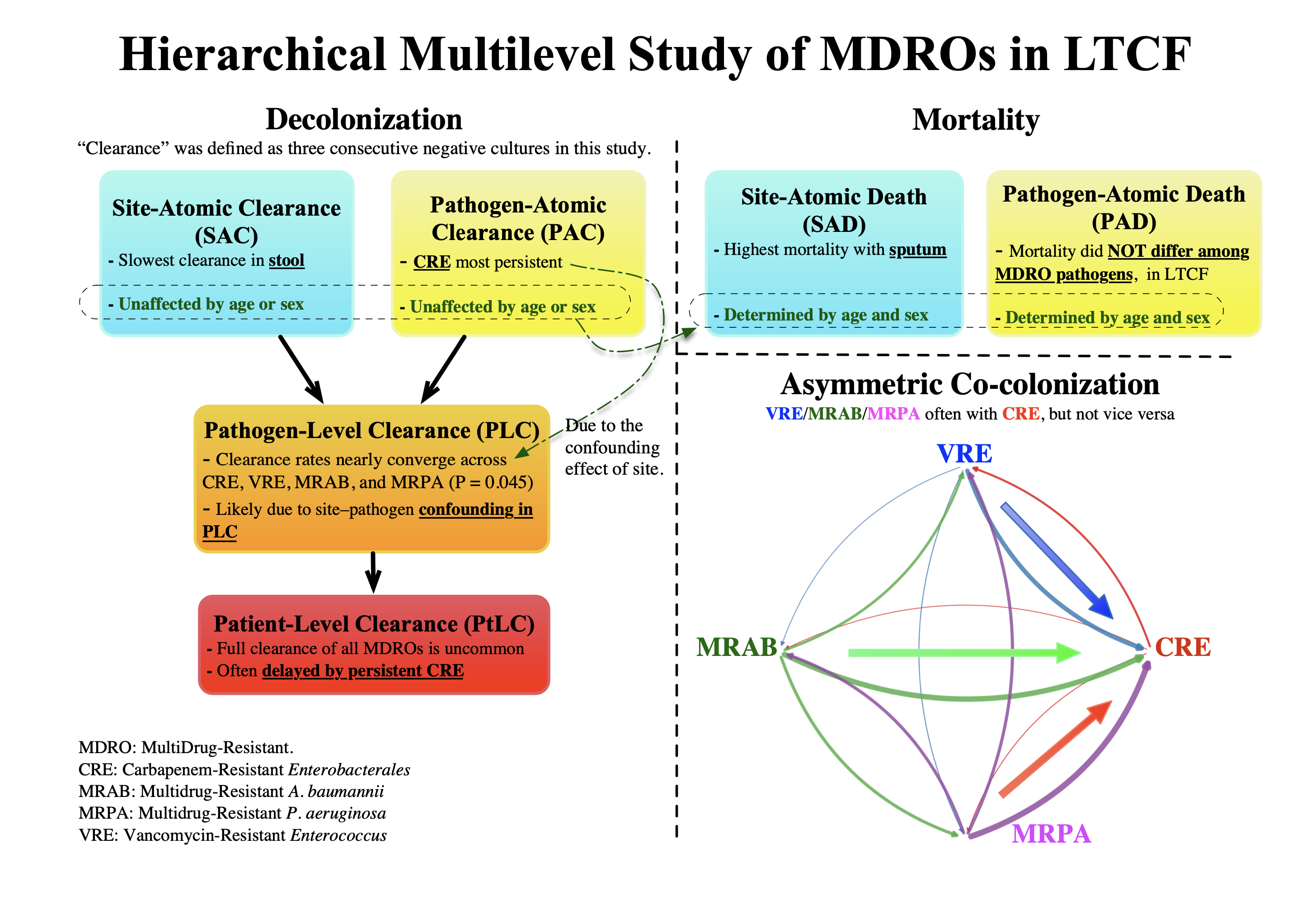
- Four-tier analysis separates site and pathogen confounding effects in decolonization
- Sputum carriage and patient factors—not pathogen—drive mortality, in LTCF
- Stool and CRE decolonize slowest, unexpectedly independent of patient age or sex
- Asymmetric co-colonization: non-CRE often with CRE, but not vice versa → screen for CRE after non-CRE isolation
- Investigate directional transmission dynamics (e.g., VRE+MRSA → VRSA)
Abstract
Background
Prior long-term-care (LTC) studies confound anatomic reservoir and pathogen effects when multiple multidrug-resistant organisms (MDROs) circulate. We created a four-tier clearance framework to disentangle site- and species-specific behavior and quantify decolonization, mortality, and asymmetric co-colonization.
Methods
Between January 2024 and May 2025, 98 LTC residents colonized with carbapenem-resistant Enterobacterales (CRE), vancomycin-resistant Enterococcus (VRE), or multidrug-resistant Pseudomonas aeruginosa (MRPA) or Acinetobacter baumannii (MRAB) underwent weekly stool, urine, sputum, wound, blood cultures, yielding a total of 2,772 specimens. Clearance—operationally defined as three consecutive negatives—was analyzed across four tiers (site-atomic, pathogen-atomic, pathogen-level, patient-level). Conditional-probability tables were constructed to summarize how frequently the four MDROs co-colonized the same patient.
Results
Clearance was slowest in stool and for CRE, independent of patient attributes of age or sex. In this LTCF cohort, mortality depended on sputum carriage and host factors rather than pathogen identity. More than half of residents carried multiple MDROs, and conditional-probability analysis revealed asymmetric co-colonization: non-CRE organisms almost always co-colonized with CRE, whereas the reverse was uncommon.
Conclusions
The hierarchical analysis showed that, contrary to common expectations, decolonization was independent of patient attributes (age and sex) and that, in this LTCF setting, mortality was unrelated to pathogen identity. Asymmetric co-colonization therefore warrants automatic CRE screening following MRAB, MRPA, or VRE isolation, and underscores the need to investigate directional co-colonization patterns among multiple MDRO co-colonizations commonly observed in LTCFs—as exemplified by vanA transfer from VRE to MRSA (methicillin-resistant Staphylococcus aureus) yielding VRSA (vancomycin-resistant Staphylococcus aureus).
Introduction
Multidrug-resistant organisms (MDRO) infections pose a critical global health threat and are associated with worse outcomes than drug-susceptible infections [1]. Although most MDRO research has focused on acute-care or tertiary hospital settings, long-term care facilities (LTCF) are increasingly recognized as significant reservoirs of resistant pathogens [2]. Outcomes of MDRO infections vary by infection site, organism type, and the presence of polymicrobial infections [3, 4]. Co-colonization—where patients harbor multiple MDROs—is being reported frequently in acute and post-acute settings, further complicating infection control and worsening clinical outcomes [5].
Prior longitudinal studies of MDRO carriage exhibit one or more of the following limitations: single‐pathogen focus, retrospective design, limited sample sizes, short‐term study periods, heterogeneous follow-up intervals, and complex symptom-driven follow-up endpoints [6-11]. More critically, they seldom account for the intertwined effects of anatomical site and pathogen, and almost never examine the directional, asymmetric co‐colonization of multiple MDROs—leaving two critical gaps unaddressed. First, intra‐patient heterogeneity is obscured: some pathogens decolonize rapidly while others prolong quarantine [11], and different anatomical sites (e.g., sputum versus stool) exhibit markedly divergent decolonization kinetics for the same pathogen [12]. Second, the asymmetric nature of co‐colonization is overlooked: the presence of one pathogen often predicts carriage of another, yet the reverse association may be weak [13].
In the absence of a routinely recommended decolonization strategy for MDRO carriage, understanding clearance dynamics is critical, as infection-control policies in LTCFs must rely on natural clearance. Building on prior work and within existing clinical constraints, a prospective cohort study was conducted in a Korean LTCF, tracking a sizable resident population over an extended period during which hundreds of adjudicated events—clearance (operationally defined here as three consecutive negative cultures), death, or censoring—were captured and classified within a four-tier analytic hierarchy to minimize confounding by anatomical reservoir and pathogen. This four-tier framework, combined with conditional-probability analysis, provides a rigorous method for quantifying decolonization dynamics, mortality, and the directional co-colonization patterns that emerge when multiple MDROs circulate.
Methods
Study design and setting
This prospective cohort study of MDRO colonization dynamics was conducted from January 2024 through May 28, 2025, at Seoul Smart Convalescent Hospital (SSCH), a LTCF in the Republic of Korea. Patients were placed in single rooms whenever possible; if capacity was exceeded, cohort isolation was applied in multi-bed rooms. Adults aged ≥18 years were enrolled if they had colonization at baseline, defined as (i) an MDRO-positive culture detected on admission screening or during symptom-driven testing within the facility, or (ii) transfer from another hospital with documented MDRO carriage. Although SSCH routinely admits patients retrospectively identified as MDRO carriers at other hospitals for quarantine, all surveillance data in this study were collected prospectively after enrollment. “Clearance” was operationally defined, per Korea Disease Control and Prevention Agency (KDCA) guidelines, as three consecutive negative cultures—each obtained at least three days apart—from every anatomic site that had previously yielded a target organism; we used this definition as a clear endpoint for observing quarantined patients. Participants were followed until clearance, death, administrative censoring on May 28, 2025, or censoring at the date of the last weekly culture due to permanent discharge, transfer without return, or withdrawal of consent, whichever occurred first. Patient attributes (age and birth-assigned biological sex) and clinical endpoints, including in-hospital death, were extracted from the electronic medical record. The Institutional Review Board of SSCH—registered with the Korean Ministry of Health and Welfare (Registration No. 3-70094812-AB-N-01)—approved the study protocol (IRB No. 2024-CR-001; approved January 2, 2024), and all participants (or their legal guardians) provided written informed consent in accordance with the Declaration of Helsinki and Korean Good Clinical Practice guidelines.
Eligibility criteria and target organisms
Eligible participants were adult inpatients colonized with at least one of four prespecified MDROs—carbapenem-resistant Enterobacterales (CRE), vancomycin-resistant Enterococcus (VRE), multidrug-resistant Pseudomonas aeruginosa (MRPA), or multidrug-resistant Acinetobacter baumannii (MRAB), where KDCA mandates isolation exclusively for CRE and leaves isolation of other MDROs to institutional discretion. Residents whose only MDRO fell outside these four categories—such as carbapenem-resistant Pseudomonas aeruginosa (CRPA) or carbapenem-resistant Acinetobacter baumannii (CRAB)—were excluded because KDCA guidelines specify MRPA and MRAB, not CRPA or CRAB, for quarantine. Species were identified by MALDI-TOF MS, and antimicrobial susceptibility testing was performed with the VITEK-2 system; interpretations followed CLSI M100 breakpoints [14].
Surveillance culture protocol
Upon first documentation of MDRO carriage, residents were enrolled in a structured surveillance program. At baseline, rectal swabs and urine cultures were obtained to screen for CRE and VRE, and urine and sputum cultures with susceptibility testing were collected for all four target organisms. Thereafter, once an anatomic site tested positive for any target MDRO, we obtained weekly rectal swabs, urine specimens, and sputum specimens from that site. Cultures were collected at least once per week, even if a resident was briefly transferred to a nearby acute-care hospital for treatment or procedure and then readmitted; this ensured at least one culture per week. Missing a weekly culture constituted an exclusion criterion; specifically, patients who could not complete uninterrupted weekly surveillance—such as those briefly transferred and readmitted—were excluded. To allow peers to examine the full culture sequence, all results have been released in Supplementary Dataset S1 (RawDataset.zip) for complete transparency and potential secondary analysis. Rigorous compliance was enforced by national policy: the Korean Health Insurance Review and Assessment Service (HIRA) withholds reimbursement for isolation care if mandated cultures are skipped. Blood and wound specimens were obtained only when clinically indicated or when a referring facility had already reported a positive result. Stool cultures were omitted for MRPA and MRAB, as these non-fermenters rarely colonize the gastrointestinal tract and prior validation studies demonstrated negligible yield [15, 16]. Each isolate was logged by pathogen, anatomic site, and collection date.
Multi-Tiered Hierarchical Clearance Classification
The tiers progress from the most granular—site-atomic clearance (SAC) and pathogen-atomic clearance (PAC)—to pathogen-level clearance (PLC) and, ultimately, patient-level clearance (PtLC). Because SAC and PAC are novel terms, detailed plain-language definitions with an illustrative example are provided in Supplementary Note S2. When multiple MDROs are present, with potential conflation between site and pathogen, SAC reflects clearance per individual site, allowing comparisons across the atomic unit of reservoir sites (stool, urine, sputum, wound, blood), whereas PAC reflects clearance with respect to pathogens, allowing comparisons across the atomic unit of the pathogen (CRE, VRE, MRAB, MRPA).
SAC is achieved when a single anatomic site yields three consecutive negative cultures for the given pathogen previously isolated, regardless of culture results from other sites for the same pathogen or from any sites for other pathogens. PAC parallels SAC but shifts the focus to the organism: a PAC event is recorded when a specific pathogen produces three consecutive negative cultures at a given site, independent of its persistence at other sites or the coexistence of other organisms. PLC aggregates all sites within a single patient for one pathogen. It is achieved when every site that ever yielded that pathogen records three consecutive negative cultures, thereby documenting eradication of that specific pathogen from the host. PtLC sits atop the hierarchy and serves as the operational trigger for discontinuing transmission-based precautions. It requires three consecutive negative cultures from every site that has ever harbored any target MDRO in that patient. Although PLC and PtLC might seem similar, they serve distinct purposes: PLC defines eradication of a particular organism from all previously positive sites in a single patient, whereas PtLC extends this concept to the global eradication of every colonizing pathogen.
Statistical Analysis
All analyses were performed using the statistical software R, version 4.4.1 (the R Foundation for Statistical Computing, Vienna, Austria) on macOS. The primary endpoint was time to clearance, measured in days from the index positive culture to the first of three consecutive negative cultures meeting the study’s clearance criteria. The secondary endpoint was all-cause, in-hospital mortality, calculated from the date of the first post-admission culture. Mortality was evaluated only at the atomic strata—site-atomic death (SAD) script and pathogen-atomic death (PAD).
Kaplan–Meier curves were generated for each hierarchical tier to characterize colonization persistence and overall survival; medians and 95 % confidence intervals (CIs) were read directly from the curves [17]. When fewer than 50 % of subjects in a stratum experienced the event, the median was reported as “not reached” (NR); when a Greenwood‐based bound could not be estimated, it was reported as “not estimable” (NE). The effects of age (continuous) and sex on clearance and mortality were assessed with Cox proportional-hazards models, and results are presented as hazard ratios (HRs) with 95 % CIs. Two-sided P values < 0.05 were considered statistically significant.
Pathogen co-colonization was examined by converting the patient-by-pathogen presence–absence matrix into a conditional-probability matrix, P(b | a), representing the probability of isolating pathogen b at any time—preceding, concurrent with, or following—the isolation of pathogen a in the same patient.
Results
Study Population and Culture Episodes
From January 2024 through May 28, 2025, the study enrolled 124 patients (Fig. 1). Twenty-six patients were excluded according to the predefined criteria described in Methods. As a result, 98 patients were included in the analysis. The majority (n = 91, 92.9 %) were transferred from a nearby hospital for isolation, while seven were identified as MDRO carriers at SSCH itself. The median age was 79.5 years (IQR, 69.0–84.0), and 50 (51.0 %) were male. Across this cohort, a total of 2,772 culture episodes were recorded: 1,776 for CRE, 632 for VRE, 133 for MRAB, and 181 for MRPA.
Site-atomic clearance (SAC)
Ninety‐eight LTCF residents generated 274 SAC episodes: stool (n = 115), urine (n = 84), sputum (n = 63), wound (n = 11), and blood (n = 2) (Table 1). Blood is shown for completeness but was excluded from modeling because no clearances or deaths occurred. Kaplan–Meier curves differed significantly across sites (Fig. 2a; log‐rank P < 0.001). Stool was the most persistent reservoir (median time‐to‐clearance, 181d; 95% CI, 134–273), whereas sputum, urine, and wound colonization cleared in median 78d (95% CI, 44–112), 47d (95% CI, 36–82), and 28d (95% CI, 21–NE [upper bound not estimable]), respectively. In a multivariable Cox model using stool as the reference (Table 2), the adjusted clearance rate ratio increased 2.66-fold for sputum (hazard ratio [HR], 2.66; 95% CI, 1.60–4.44), 2.84-fold for urine (HR, 2.84; 95% CI, 1.83–4.40), and 5.25-fold for wounds (HR, 5.25; 95% CI, 2.50–10.99); neither age (HR, 0.999; 95% CI, 0.984–1.014) nor sex (male HR, 1.16; 95% CI, 0.80–1.67) was independently associated with clearance. At the SAC tier, stool exhibited the slowest clearance with marked variation across sites, and clearance was independent of patient age and sex.
Site-atomic death (SAD)
During the same interval, 88 of the 274 site-atomic episodes ended in death (Fig. 2b). Median survival differed significantly by anatomical site (log-rank P = 0.02): it was shortest for sputum-colonized residents (median, 68d; 95% CI, 51–NE), intermediate for stool (144d; 95% CI, 93–244), and longest for urine (189d; 95% CI, 155–NE); wound and blood episodes were too sparse for reliable estimates. In the fully adjusted Cox model using sputum as the reference (Table 2), stool carriage was associated with a 41% lower mortality hazard (HR, 0.59; 95% CI, 0.36–0.97) and urine carriage with a 51% lower hazard (HR, 0.49; 95% CI, 0.26–0.92); the wound–sputum contrast did not reach statistical significance (HR, 0.42; 95% CI, 0.05–3.14). Each additional year of age increased the risk of death by 4.4% (HR, 1.044; 95% CI, 1.022–1.067), and male sex conferred a 90% excess hazard (HR, 1.91; 95% CI, 1.23–2.96). At the SAD tier, mortality was highest in sputum-colonized residents, varied significantly by site, and—unlike clearance—was influenced by age and sex.
Pathogen-atomic clearance (PAC)
All 274 PAC episodes—CRE (n = 156), VRE (n = 68), MRPA (n = 29), and MRAB (n = 21)—were evaluable (Table 1). Kaplan–Meier curves separated sharply by pathogen (Fig. 2c; log-rank P ≈ 1 × 10⁻⁹). CRE was the most tenacious organism, with a median time-to-clearance of 159d (95% CI, 111–246) and a crude clearance rate of 32.1%. In contrast, MRAB cleared in a median 28d (95% CI, 26–NE) with a 76.2% clearance rate; MRPA cleared in 27d (95% CI, 24–94) with a 69.0% rate; and VRE cleared in 61d (95% CI, 51–139) with a 51.5% rate. In a multivariable Cox model using CRE as the reference (Table 2), the adjusted clearance rate ratio was 5.30-fold higher for MRAB (HR, 5.30; 95% CI, 2.96–9.51), 5.12-fold higher for MRPA (HR, 5.12; 95% CI, 3.00–8.75), and 2.04-fold higher for VRE (HR, 2.04; 95% CI, 1.32–3.16); neither age (HR, 0.9965; 95% CI, 0.981–1.012) nor male sex (HR, 1.09; 95% CI, 0.76–1.58) was significant. At the PAC tier, CRE cleared most slowly, VRE intermediately, and MRAB/MRPA cleared fastest; as at the SAC tier, clearance was independent of patient age and sex.
Pathogen-atomic death (PAD)
Of the 274 pathogen-atomic episodes, 88 ended in death (Fig. 2d; log-rank P = 0.80), and the survival curves for CRE, VRE, MRAB, and MRPA were virtually identical. Median survival was 136d (95% CI, 102–189) for CRE and 293d (95% CI, 89–NE) for VRE; medians for MRAB and MRPA were not reached (lower 95% CI bound NE for MRAB and 41 d for MRPA). In a fully adjusted Cox model (Table 2), none of the non-CRE pathogens—MRAB (HR, 0.98; 95% CI, 0.30–3.20), MRPA (HR, 0.90; 95% CI, 0.36–2.27), or VRE (HR, 0.82; 95% CI, 0.48–1.41)—significantly affected mortality risk compared with CRE. Instead, host factors predominated: each additional year of age increased the mortality hazard by 4.8% (HR, 1.048; 95% CI, 1.025–1.071), and male sex conferred a 92% excess hazard (HR, 1.92; 95% CI, 1.24–2.98). At the PAD tier, no specific organism uniquely predicted death in our LTCF cohort; instead, mortality was driven by host factors (age and sex). Notably, clearance at the SAC and PAC tiers was independent of those patient attributes.
Pathogen-level clearance (PLC)
The cohort generated 173 PLC episodes—CRE (n = 85), VRE (n = 44), MRPA (n = 23), and MRAB (n = 21)—of which 14/85 (16.5%), 17/44 (38.6%), 16/23 (69.6%), and 14/21 (66.7%) met the clearance definition, respectively (Table 1). Median time-to-clearance was 68 d (95% CI, 53–246) for CRE, 57d (95% CI, 41–139) for VRE, 26d (95% CI, 21–94) for MRPA, and 28d (95% CI, 27–78) for MRAB. Kaplan–Meier curves appeared broadly similar (Fig. 2e), and the global log-rank test indicated modest differences among pathogens (P = 0.0397). Thus, unlike the PAC tier—where clearance kinetics varied sharply by species (log-rank P ≈ 1 × 10⁻⁹)—aggregation at the PLC tier attenuates but does not entirely eliminate those differences, as reflected by the more modest global log-rank P value of 0.0397, which only just meets the conventional 0.05 threshold.
Patient-level clearance (PtLC)
Complete PtLC remained uncommon: 18 events occurred among 17 of 98 residents (18.4%), who achieved three consecutive negative cultures at all previously positive sites (Table 1). As shown in Fig. 1, one resident (patient 1004) reached PtLC twice—first after multi-MDRO clearance and again following re-isolation. The overall median time to PtLC was 97 d (95 % CI, 53–238; Fig. 2f), exceeding the pathogen-level medians for CRE (68 d), VRE (57 d), MRPA (26 d), and MRAB (28 d), as PtLC incorporates clearance across all four MDROs and thus cannot be shorter than any individual PLC.
Co-colonization profile
The upper panel of Table 3 shows patient counts. Among the 98 residents, CRE remained the dominant organism, colonizing 80 individuals (81.6%), whereas VRE, MRAB, and MRPA were present in 42.9%, 17.3%, and 19.4%, respectively. Co-carriage was common: 49 residents (50.0%) harbored at least two target MDROs, and 18 (18.4%) carried three or more, underscoring the polymicrobial pressure typical of long-term care. The most frequent dyad was CRE + VRE (27 of 98, 27.6%), followed by CRE + MRPA (16 of 98, 16.3%) and CRE + MRAB (13 of 98, 13.3%); no other pair exceeded 10% prevalence.
Notably, the lower panel of Table 3 presents a strongly asymmetric co-colonization network centered on CRE: 76.5 % of MRAB carriers and 84.2 % of MRPA carriers were also colonized with CRE, whereas the reverse probabilities were only 16.2 % and 20.0 %, respectively. For transparency, patient-level co-colonization profiles are provided in Supplementary Table S3.

Discussion
The present study refines our understanding of colonization dynamics in LTCFs by introducing a four-tier hierarchical framework—SAC, PAC, PLC, and PtLC—to disentangle clearance kinetics. At the PLC tier, organism‐specific differences in clearance are substantially attenuated but not eliminated (log-rank P = 0.0397), contrasting sharply with the highly significant differences observed at the PAC tier (log-rank P ≈ 1 × 10⁻⁹) and confirming that this additional stratification mitigates reservoir-driven confounding. This occurs because PLC has an intrinsic limitation: by aggregating sites and pathogens, it requires every previously culture-positive site to register three consecutive negative cultures. For example, CRE’s PLC can be substantially delayed by persistent stool colonization, even though sputum colonization clears much more quickly. To address this confounding, the PAC and SAC tiers were devised to focus separately on pathogen and site, respectively. The PAC tier captures intrinsic species behavior across sites, showing that some organisms (e.g., VRE) clear rapidly regardless of location, whereas others (e.g., CRE) persist. Prior reports confirm this pattern: 87.5% of VRE carriers had cleared compared with only 50% of CRE carriers [18], median ~26 weeks for VRE [19], while ~65% of CRE carriers remained colonized at one year [20]. These differences likely reflect ecological factors, as CRE persist within the colonic mucus layer whereas VRE are excluded [21]. The SAC tier provides a site-specific perspective: stool cultures clear extraordinarily slowly, reflecting the gut’s role as a protected reservoir where MDROs persist [6, 8], whereas sputum and urine often convert quickly because non-GI sites are more responsive to source control and local interventions [9, 10]—contrasts that PLC or PtLC would mask. For example, in patients with IDs 1023 and 1076, stool clearance was markedly delayed, while multiple urine sites cleared rapidly.
One might be tempted to attribute mortality to the colonizing pathogen, but when the intertwined confounding effects of anatomic site and species are disentangled, this assumption does not hold in an LTCF setting. PAD-tier survival curves for CRE, VRE, MRAB, and MRPA were nearly superimposable (log-rank P = 0.80; Fig. 2d), suggesting that no organism carried a significantly different mortality risk. This finding is plausible because LTCF residents are often chronically colonized with MDROs or merely isolated and quarantined without overt infection symptoms, meaning these pathogens contribute little to mortality. These results underscore that, in LTCFs, although organism-centered measures remain critical for transmission prevention and mortality prediction, improving survival hinges on addressing host factors (advanced age and male sex) and site-specific vulnerabilities—particularly sputum carriage—rather than solely targeting individual pathogens.
Patient attributes—age and sex—were significant predictors of mortality at both the SAD and PAD tiers. Although one might intuitively link age and sex to clearance, our study demonstrates the opposite: at both the SAC and PAC tiers, clearance was independent of these patient attributes, a distinction that can inform discussions with patients and caregivers—for example, those who wonder whether their elderly parent can be decolonized. This likely reflects that clearance is driven by local microbiological and environmental dynamics—biofilm architecture, microbiome composition, antibiotic pressure, and tissue comorbidities [8, 22, 23]—none of which correspond closely to systemic immunosenescence or sex-based immune differences.
This study has several limitations. First, our clearance definition was calibrated to Korean national regulations, which may limit generalizability to other settings. Second, follow-up began with the first positive culture at our facility, which may not represent the true onset of colonization; some residents were already colonized before admission, so carriage duration may have been underestimated. Third, universal baseline screening from negative through acquisition to clearance was not performed and was impractical in our LTCF setting: in Korea, isolation care is reimbursed fee-for-service, while non-isolation long-term care is largely reimbursed under a bundled payment system. Once acquisition is documented, caregivers expect serial cultures to enable isolation release, but they generally resist pre-acquisition screening because it could trigger quarantine, and hospitals must absorb the cost under bundled payment models. There is limited incentive on either side, making universal surveillance infeasible.
In this real-world context, automatic CRE screening after MRAB, MRPA, or VRE serves as a pragmatic alternative to universal surveillance. As shown in Table 3, co-colonization was strongly asymmetric. Because our conditional probabilities are longitudinal rather than contemporaneous at the trigger event, they do not themselves yield a cross-sectional number-needed-to-test (NNT). Nonetheless, more than three-quarters of MRAB carriers (76.5%) and over four-fifths of MRPA carriers (84.2%) also harbored CRE, whereas only 16.2% of CRE carriers had MRAB and 20.0% had MRPA. For facilities without active surveillance, this translates into targeted CRE screening with a single batched culture run for the flagged subset, reducing both nursing effort and laboratory costs compared with universal screening. Beyond this practical application, it remains essential to investigate directional dynamics more broadly: horizontal transfer of vanA from VRE to MRSA has produced de novo VRSA in co-colonized patients [24]. Such cases demonstrate how simultaneous colonization within the same niche facilitates gene transfer, underscoring the directional and asymmetric nature of these interactions.
In conclusion, this study offers a distinctive contribution by pairing a four-tier hierarchical framework with conditional-probability mapping to disentangle the often-confounded influences of pathogen and anatomic site in LTCFs—an angle rarely explored in previous MDRO research. It overturns intuitive expectations by showing that, in this LTCF, mortality depends more on colonization site than on pathogen identity (MDROs here are often detected as chronic colonizers rather than causing acute illness), whereas clearance is independent of patient attributes such as age and sex—a finding that may reassure caregivers worried that advanced age impedes decolonization. The asymmetric co-colonization pattern we uncovered—non-CRE organisms almost always co-colonized with CRE, whereas CRE carriers rarely host other MDROs—supports automatic CRE screening whenever MRPA, MRAB, or VRE is detected and further highlights the need for systematic investigation of directional co-colonization dynamics—such as transfer of vanA from VRE to MRSA leading to de novo VRSA, thereby increasing P(VRSA | VRE + MRSA)—in LTCFs burdened by multiple MDROs.
References
[1] EclinicalMedicine: Antimicrobial resistance: a top ten global public health threat. EClinicalMedicine 2021;41: 101221.
[2] O'Fallon E, Pop-Vicas A, D'Agata E: The emerging threat of multidrug-resistant gram-negative organisms in long-term care facilities. J Gerontol A Biol Sci Med Sci 2009;64(1): 138-141.
[3] Centers for Disease C, Prevention: Vital signs: carbapenem-resistant Enterobacteriaceae. MMWR Morbidity and mortality weekly report 2013;62(9): 165-170.
[4] Cilloniz C, Calabretta D, Palomeque A, Gabarrus A, Ferrer M, Marcos MA, et al.: Risk Factors and Outcomes Associated With Polymicrobial Infection in Community-Acquired Pneumonia. Arch Bronconeumol 2025.
[5] Tadese BK, DeSantis SM, Mgbere O, Fujimoto K, Darkoh C: Clinical Outcomes Associated with Co-infection of Carbapenem-Resistant Enterobacterales and other Multidrug-Resistant Organisms. Infect Prev Pract 2022;4(4): 100255.
[6] Mo Y, Hernandez-Koutoucheva A, Musicha P, Bertrand D, Lye D, Ng OT, et al.: Duration of Carbapenemase-Producing Enterobacteriaceae Carriage in Hospital Patients. Emerg Infect Dis 2020;26(9): 2182-2185.
[7] Nutman A, Lerner A, Fallach N, Schwartz D, Carmeli Y: Likelihood of persistent carriage of carbapenem-resistant Acinetobacter baumannii on readmission in previously identified carriers. Infect Control Hosp Epidemiol 2019;40(10): 1188-1190.
[8] Byers KE, Anglim AM, Anneski CJ, Farr BM: Duration of colonization with vancomycin-resistant Enterococcus. Infect Control Hosp Epidemiol 2002;23(4): 207-211.
[9] Haverkate MR, Derde LP, Brun-Buisson C, Bonten MJ, Bootsma MC: Duration of colonization with antimicrobial-resistant bacteria after ICU discharge. Intensive Care Med 2014;40(4): 564-571.
[10] Pacio GA, Visintainer P, Maguire G, Wormser GP, Raffalli J, Montecalvo MA: Natural history of colonization with vancomycin-resistant enterococci, methicillin-resistant Staphylococcus aureus, and resistant gram-negative bacilli among long-term-care facility residents. Infect Control Hosp Epidemiol 2003;24(4): 246-250.
[11] Lin I-W, Huang C-Y, Pan S-C, Chen Y-C, Li C-M: Duration of colonization with and risk factors for prolonged carriage of multidrug resistant organisms among residents in long-term care facilities. Antimicrobial Resistance & Infection Control 2017;6.
[12] Zirakzadeh A, Patel R: Vancomycin-resistant enterococci: colonization, infection, detection, and treatment. Mayo Clin Proc 2006;81(4): 529-536.
[13] Heinze K, Kabeto M, Martin ET, Cassone M, Hicks L, Mody L: Predictors of methicillin-resistant Staphylococcus aureus and vancomycin-resistant enterococci co-colonization among nursing facility patients. Am J Infect Control 2019;47(4): 415-420.
[14] Institute CaLS. Performance Standards for Antimicrobial Susceptibility Testing. Wayne, PA. 2023.
[15] Lortholary O, Fagon JY, Buu Hoi A, Mahieu G, Gutmann L: Colonization by Acinetobacter baumanii in intensive-care-unit patients. Infect Control Hosp Epidemiol 1998;19(3): 188-190.
[16] Estepa V, Rojo-Bezares B, Torres C, Saenz Y: Faecal carriage of Pseudomonas aeruginosa in healthy humans: antimicrobial susceptibility and global genetic lineages. FEMS Microbiol Ecol 2014;89(1): 15-19.
[17] Kleinbaum DG, Klein M. Survival Analysis: A self-Learning Text. LLC, 233 Spring Street, New York, NY 10013, USA: Springer Science + Business Media. 2012.
[18] Dinh A, Fessi H, Duran C, Batista R, Michelon H, Bouchand F, et al.: Clearance of carbapenem-resistant Enterobacteriaceae vs vancomycin-resistant enterococci carriage after faecal microbiota transplant: a prospective comparative study. J Hosp Infect 2018;99(4): 481-486.
[19] Shenoy ES, Paras ML, Noubary F, Walensky RP, Hooper DC: Natural history of colonization with methicillin-resistant Staphylococcus aureus (MRSA) and vancomycin-resistant Enterococcus (VRE): a systematic review. BMC Infect Dis 2014;14: 177.
[20] Bar-Yoseph H, Hussein K, Braun E, Paul M: Natural history and decolonization strategies for ESBL/carbapenem-resistant Enterobacteriaceae carriage: systematic review and meta-analysis. J Antimicrob Chemother 2016;71(10): 2729-2739.
[21] Caballero S, Carter R, Ke X, Susac B, Leiner IM, Kim GJ, et al.: Distinct but Spatially Overlapping Intestinal Niches for Vancomycin-Resistant Enterococcus faecium and Carbapenem-Resistant Klebsiella pneumoniae. PLoS Pathog 2015;11(9): e1005132.
[22] Ciobotaro P, Flaks-Manov N, Oved M, Schattner A, Hoshen M, Ben-Yosef E, et al.: Predictors of Persistent Carbapenem-Resistant Enterobacteriaceae Carriage upon Readmission and Score Development. Infect Control Hosp Epidemiol 2016;37(2): 188-196.
[23] Seong H, Lee SK, Cheon JH, Yong DE, Koh H, Kang YK, et al.: Fecal Microbiota Transplantation for multidrug-resistant organism: Efficacy and Response prediction. J Infect 2020;81(5): 719-725.
[24] Marchaim D, Perez F, Lee J, Bheemreddy S, Hujer AM, Rudin S, et al.: "Swimming in resistance": Co-colonization with carbapenem-resistant Enterobacteriaceae and Acinetobacter baumannii or Pseudomonas aeruginosa. Am J Infect Control 2012;40(9): 830-835.
© 2025 King Saud Bin Abdulaziz University for Health Sciences.
Licensed under
CC BY 4.0.
Pulmonary resection for multidrug-resistant tuberculosis: systematic review and meta-analysis
Hyunsuk Frank Roh, MD; Jihoon Kim, MD;
Seung Hyuk Nam, MD; and Jung Mogg Kim, MD, PhD
DOI:
https://doi.org/10.1093/ejcts/ezx209
Highlights
- Pulmonary resection improves survival when combined with optimized MDR-TB chemotherapy
- Surgical candidates benefit most when sputum conversion is incomplete or disease burden is extensive
- Different resection types (wedge, segmentectomy, lobectomy) demonstrate comparable mortality when appropriately selected
- Adverse events remain acceptable when surgery is performed in high-volume thoracic centers
- Meta-analytic evidence supports surgery as an adjunct—not replacement—to standard MDR-TB medical therapy

Piperacillin-tazobactam versus meropenem for ceftriaxone-resistant Enterobacterales bacteremia: visual synthesis across key studies
The clearest head-to-head comparison for piperacillin-tazobactam (pip/tazo) in ceftriaxone-resistant E. coli or K. pneumoniae bacteremia comes from a randomized trial (MERINO), in which 30-day mortality was higher with pip/tazo than with meropenem.
Earlier observational cohorts comparing carbapenems with pip/tazo or broader BLBLI therapy showed mixed signals, largely in parallel with substantial differences in baseline severity and infection source distribution.
I. At-a-glance dashboard
Central head-to-head question
Pip/tazo vs meropenem
Ceftriaxone-resistant E. coli or K. pneumoniae bacteremia (randomized trial)
Primary mortality signal (MERINO)
+8.6% absolute
30-day mortality: 12.3% vs 3.7% (pip/tazo minus meropenem)
Observational context (two cohorts)
Mixed
Adjusted hazard ratio estimates ranged from neutral to harmful for BLBLI/pip-tazo vs carbapenems
| Study (year) |
Design focus |
Comparator framing |
Main pip/tazo (or BLBLI) signal |
Best single takeaway |
| Harris (MERINO), 2018 |
Randomized clinical trial |
Pip/tazo vs meropenem |
Higher mortality with pip/tazo |
Meropenem demonstrated a materially lower 30-day mortality than pip/tazo in the randomized comparison. |
| Tamma, 2015 |
Retrospective cohort (higher acuity) |
Pip/tazo vs carbapenem |
Harm signal for pip/tazo |
Adjusted results suggested higher hazard of death with pip/tazo in a higher-severity cohort. |
| Rodriguez-Baño, 2012 |
Retrospective cohort (lower acuity) |
BLBLI vs carbapenem |
No detected harm (wide CI) |
In a predominantly low-severity, urinary/biliary-source cohort, BLBLI definitive therapy did not show an excess mortality signal after adjustment. |
II. Central evidence: Harris (MERINO) randomized trial emphasizing pip/tazo versus meropenem
Primary endpoint (30-day mortality)
- Primary analysis: pip/tazo 23/187 (12.3%) vs meropenem 7/191 (3.7%).
- Absolute risk difference: +8.6% (pip/tazo minus meropenem), approximately 1 additional death per ~12 treated (derived from the displayed counts).
- Per-protocol analysis: pip/tazo 18/170 (10.6%) vs meropenem 7/186 (3.8%), absolute difference +6.8%.
30-day mortality (primary analysis) — bar lengths scaled to 15%
Piperacillin-tazobactam
12.3% (23/187)
Visual scaling note: 15% corresponds to 100% bar width to improve legibility of low event rates.
30-day mortality (per-protocol) — bar lengths scaled to 15%
Piperacillin-tazobactam
10.6% (18/170)
These two panels show consistent directionality (higher mortality with pip/tazo) across analytic sets.
Secondary endpoints displayed in the trial summary table
- The displayed endpoints include early clinical/microbiological success and specific failure events (microbiological relapse; secondary infection with multidrug-resistant organisms or C. difficile).
- Directional differences favored meropenem for early success metrics and favored meropenem for failure-event rates, with confidence intervals presented as broad for several endpoints.
| Endpoint (as displayed) |
Pip/tazo |
Meropenem |
Between-group difference (pip/tazo − meropenem) |
| Clinical and microbiological success at day 4 |
121/177 (68.4%) |
138/185 (74.6%) |
-6.2% (95% CI -15.5 to 3.1) |
| Microbiological success at day 4 |
169/174 (97.1%) |
184/185 (99.5%) |
-2.3% (95% CI -6.1 to 0.4) |
| Microbiological relapse |
9/187 (4.8%) |
4/191 (2.1%) |
+2.7% (95% CI -1.1 to 7.1) |
| Secondary infection with multidrug-resistant organism or C. difficile |
15/187 (8.0%) |
8/191 (4.2%) |
+3.8% (95% CI -1.1 to 9.1) |
III. Observational comparison to support interpretation: Tamma (2015) and Rodriguez-Baño (2012)
Effect-size visualization (adjusted hazard ratios versus carbapenems)
- The following graphic summarizes adjusted hazard ratio point estimates and confidence intervals shown in the slide tables, using a shared scale from 0 to 4.
- The vertical reference line marks HR = 1.0 (no difference); points to the right suggest higher hazard with pip/tazo or BLBLI therapy, while points to the left suggest lower hazard.
0
1
2
3
4
Rodriguez-Baño 2012 (BLBLI vs carbapenem)
HR 0.76 (0.28–2.07)
Tamma 2015 (pip/tazo vs carbapenem)
HR 1.92 (1.07–3.45)
Visual scaling note: the axis is fixed at 0–4 for both rows; confidence intervals extending beyond the axis would be truncated (not applicable to the displayed values).
Case-mix contrasts that plausibly drive discordant observational signals
- Rodriguez-Baño cohort: predominantly E. coli, urinary/biliary sources ~68%, Pitt score median ~1, ICU admission ~8.7%, neutropenia ~4.8%.
- Tamma cohort: mixed pathogens (E. coli, K. pneumoniae, Proteus), urinary/biliary sources ~30%, Pitt score mean ~2.2, ICU admission ~33.8%, neutropenia ~15%.
- These contrasts align with a common pattern in severe infection therapeutics: higher acuity and less favorable sources increase the clinical penalty of marginal pharmacodynamic performance.
| Dimension |
Rodriguez-Baño 2012 (lower acuity profile) |
Tamma 2015 (higher acuity profile) |
Interpretive implication |
| Organisms |
Primarily E. coli |
E. coli, K. pneumoniae, Proteus |
Greater heterogeneity may shift MIC distributions and reduce the efficacy margin for pip/tazo. |
| Urinary/biliary source proportion |
~68% |
~30% |
More non-urinary sources may correlate with higher inoculum and more complex source control. |
| Baseline severity |
Pitt median ~1; ICU ~8.7% |
Pitt mean ~2.2; ICU ~33.8% |
Effect modification by acuity can amplify an empirical advantage for carbapenems. |
| Neutropenia |
~4.8% |
~15% |
Immunosuppression increases consequence of delayed or insufficient bactericidal exposure. |
| Adjusted treatment estimate |
BLBLI: HR 0.76 (0.28–2.07) |
Pip/tazo: HR 1.92 (1.07–3.45) |
Opposing point estimates appear consistent with different case-mix rather than a true contradiction. |
IV. Integrated conclusion centered on pip/tazo head-to-head evidence
What the evidence most directly suggests about pip/tazo versus meropenem
- The randomized MERINO comparison showed higher 30-day mortality with pip/tazo than with meropenem in ceftriaxone-resistant E. coli or K. pneumoniae bacteremia.
- Within the displayed secondary outcomes, early success favored meropenem directionally, while relapse and secondary infection rates were numerically higher with pip/tazo (with wide intervals for several endpoints).
How the observational landscape fits around the randomized signal
- Observational cohorts showed mixed results: a low-acuity, source-favorable cohort appeared compatible with no excess mortality using BLBLI definitive therapy, whereas a higher-acuity cohort showed an adjusted harm signal for pip/tazo.
- The randomized trial aligns more closely with the higher-acuity harm-signal direction than with the low-acuity neutral-signal direction.
Practical takeaway (risk-stratified, humble framing)
- For ceftriaxone-resistant or ESBL-grade bacteremia, meropenem (carbapenem therapy) appears to have the most robust supportive signal when a direct comparison to pip/tazo is prioritized.
- Any carbapenem-sparing use of pip/tazo or other BLBLI therapy appears most defensible only in carefully selected, lower-risk patterns resembling the low-acuity observational cohort case-mix (favorable sources and clinical stability), while acknowledging that randomized evidence has demonstrated meaningful mortality separation in the head-to-head setting.
- This synthesis is intended for educational discussion; individual management decisions should reflect patient-specific severity, infection source, microbiologic details, dosing strategy, and local policies.
Abbreviations
- pip/tazo: piperacillin-tazobactam
- BLBLI: β-lactam/β-lactamase inhibitor
- ESBL: extended-spectrum β-lactamase
- CI: confidence interval
- HR: hazard ratio
V. References
- Harris PNA, Tambyah PA, Lye DC, et al. Effect of piperacillin-tazobactam vs meropenem on 30-day mortality for patients with E. coli or K. pneumoniae bloodstream infection and ceftriaxone resistance: a randomized clinical trial. JAMA. 2018;320:984-994.
- Tamma PD, Han JH, Rock C, et al. Carbapenem therapy is associated with improved survival compared with piperacillin-tazobactam for patients with extended-spectrum β-lactamase bacteremia. Clinical Infectious Diseases. 2015;60:1319-1325.
- Rodríguez-Baño J, Navarro MD, Retamar P, et al. β-Lactam/β-lactamase inhibitor combinations for the treatment of bloodstream infections due to extended-spectrum β-lactamase–producing Escherichia coli. Clinical Infectious Diseases. 2012;54:167-174.
Written on December 4, 2025
R-Script
Survival Analysis-Based Quarantine Clearance Prototype
Table of Contents
- Mathematical Foundation
- Survival Function and Hazard Function
- Kaplan-Meier Estimator
- Cox Proportional Hazards Model
- Fine-Gray Model for Competing Risks
- Code and Step-by-Step Explanation
-
0.
Install and Load Required Packages
-
1.
Define Output Directory
-
2.
Data Import and Preparation
-
3.
Exploratory Data Analysis (EDA)
-
4.
Kaplan-Meier Plots Stratified by Site
-
5.
Cox Proportional Hazards Model Including Site
-
6.
Checking for Multicollinearity
-
7.
Penalized Cox Regression (Lasso)
-
8.
Fine-Gray Model for Competing Risks
-
9.
Visualizing Survival Differences Across Sites
-
10.
Additional Recommendations and Checks
-
11.
End of Script
1. Mathematical Foundation
1.1. Survival Function and Hazard Function
- Survival Function \( S(t) \) is defined as:
\[
S(t) = P(T > t),
\]
where \( T \) is the random variable representing the time to event (clearance). \( S(t) \) describes the probability that a subject remains non-cleared (has not yet achieved three consecutive negative tests) after time \( t \).
- Hazard Function \( \lambda(t) \) is defined as:
\[
\lambda(t) = \lim_{\Delta t \to 0} \frac{P(t \le T < t + \Delta t \mid T \ge t)}{\Delta t}.
\]
It represents the instantaneous rate of achieving clearance at time \( t \), given that the patient has not cleared the pathogen before \( t \).
1.2. Kaplan-Meier Estimator
The Kaplan-Meier (KM) estimator is a non-parametric statistic used to estimate the survival function \( S(t) \). If there are \( n \) subjects, let \( t_{(1)}, t_{(2)}, \dots, t_{(k)} \) be the distinct event times in ascending order. Let \( d_j \) be the number of events (clearances) at time \( t_{(j)} \) and \( r_j \) be the number of subjects at risk just before \( t_{(j)} \). The KM estimator is:
\[
\hat{S}(t)
= \prod_{t_{(j)} \le t} \left( 1 - \frac{d_j}{r_j} \right).
\]
It allows comparing the time to clearance across different sites (e.g., stool vs. urine).
1.3. Cox Proportional Hazards Model
The Cox Proportional Hazards model expresses the hazard function for individual \( i \) as:
\[
\lambda_i(t) = \lambda_0(t) \exp\left( \boldsymbol{\beta}^\top \mathbf{x}_i \right),
\]
where
- \( \lambda_0(t) \) is the baseline hazard function (unspecified),
- \( \mathbf{x}_i \) is the vector of covariates (e.g., site, age, gender),
- \( \boldsymbol{\beta} \) is the vector of coefficients.
A hazard ratio between two covariate levels reflects the ratio of their hazards at any given time \( t \). If a coefficient \( \beta_j \) is positive, it suggests an increased rate of clearance for that factor level.
1.4. Fine-Gray Model for Competing Risks
When multiple competing events can occur (e.g., clearance is the event of interest, but death or loss to follow-up might preclude clearance), a competing risk model such as Fine and Gray is used:
\[
\text{Fine-Gray: } \quad \text{Subdistribution hazard } = h_j(t) = \lim_{\Delta t \to 0}
\frac{P(t \le T < t + \Delta t, \epsilon = j \mid T \ge t \text{ or } (T < t \text{ and } \epsilon \neq j))}{\Delta t},
\]
where \( \epsilon \) indicates the type of event (\( j = \) clearance, other = competing events). This method accounts for the fact that once a competing event (e.g., death) happens, one can no longer clear the pathogen.
2. Code and Step-by-Step Explanation
| Step |
Section |
Purpose |
| 0 |
Install Packages |
Ensures necessary packages are installed |
| 1 |
Define Directory |
Output directory for storing analysis results |
| 2 |
Data Import/Prep |
Loads and cleans the data |
| 3 |
Exploratory Analysis |
Summaries and missing data checks |
| 4 |
Kaplan-Meier Analysis |
Non-parametric survival estimates by site |
| 5 |
Cox Model (Simple) |
Estimates hazard ratios for clearance with Site only |
| 6 |
Multicollinearity Check |
Detects correlated predictors using VIF |
| 7 |
Penalized Cox (Lasso) |
Regularization to handle many or correlated predictors |
| 8 |
Fine-Gray Model |
Competing risks approach for clearance vs. death |
| 9 |
Visualization |
Visual compares survival curves by site |
| 10 |
Recommendations/Checks |
Influential points, outliers, and missing data |
| 11 |
End of Script |
Wrap-up, optional housekeeping |
Note: The code presented here is R-based and uses packages such as survival, survminer, cmprsk, dplyr, ggplot2, and glmnet. Adjust package calls as needed for local environment.
2.0. Install and Load Required Packages
# -------------------------------------------
# Survival Analysis on Quarantine Clearance
# Comparing Site-Specific Clearance: Stool, Urine, Sputum, Blood
# © 2024 Hyunsuk Frank Roh, MD. All rights reserved.
# -------------------------------------------

# 0. Setup: Install and Load Required Packages
install_and_load <- function(package) {
  if (!require(package, character.only = TRUE)) {
    install.packages(package, dependencies = TRUE)
    library(package, character.only = TRUE)
  }
}

required_packages <- c("survival", "survminer", "cmprsk", "dplyr", "readr",
                       "ggplot2", "patchwork", "forcats", "reshape2", "glmnet", "car")

# Load dplyr early to avoid conflicts
suppressMessages(library(dplyr))

invisible(lapply(required_packages, install_and_load))
Interpretation:
- This section ensures that all required packages for reading data, plotting, modeling, and statistical testing are present and loaded.
- Automated checks help avoid missing dependencies during runtime.
2.1. Define Output Directory
# 1. Define Output Directory
desktop_path <- file.path(Sys.getenv("USERPROFILE"), "Desktop")
output_dir <- file.path(desktop_path, "Survival_Analysis_Images")

if (!dir.exists(output_dir)) {
  dir.create(output_dir, recursive = TRUE)
  message(paste("Created directory:", output_dir))
} else {
  message(paste("Directory already exists:", output_dir))
}
Interpretation:
- Specifies where plots and model summaries will be stored.
- Recursive creation of directories ensures sub-directories exist when writing outputs.
2.2. Data Import and Preparation
# 2. Data Import and Preparation
data_path <- file.path(desktop_path, "dataset05.csv")
my_data <- read_csv(data_path, locale = locale(encoding = "UTF-8"))

cat("First few rows of the dataset:\n")
print(head(my_data))

cat("Structure of the dataset:\n")
print(str(my_data))

# Convert variables to appropriate data types
my_data <- my_data %>%
  mutate(
    PatientID = as.factor(PatientID),
    Pathogen = as.factor(Pathogen),
    Site = as.factor(Site),
    Start_Date = as.Date(Start_Date, format = "%m/%d/%Y"),
    Event_Date = as.Date(Event_Date, format = "%m/%d/%Y"),
    Event_Type = as.factor(Event_Type),
    Event_Code = as.numeric(Event_Code),
    Age = as.numeric(Age),
    Gender = as.factor(Gender),
    FactorA = as.factor(FactorA),
    FactorB = as.factor(FactorB),
    FactorC = factor(FactorC, levels = c("Low", "Medium", "High"), ordered = TRUE)
  )

cat("Structure after type conversions:\n")
print(str(my_data))
Interpretation:
- Reads the CSV file containing survival (clearance) data and sets correct data types for key variables.
- Event_Code should indicate whether an event (clearance) occurred (e.g., 1 = clearance, 0 = censored, 2 = competing event if used).
- This step ensures subsequent survival analysis is consistent with R’s expectations for times, events, and factors.
2.3. Exploratory Data Analysis (EDA)
# 3. Exploratory Data Analysis (EDA)
cat("Summary statistics:\n")
print(summary(my_data))

cat("Missing values per column:\n")
print(sapply(my_data, function(x) sum(is.na(x))))

cat("Event distribution across sites:\n")
print(table(my_data$Site, my_data$Event_Code))
Interpretation:
- Summary statistics and missing value checks identify potential data issues.
- A two-way table with Site vs. Event_Code reveals how many clearance events occurred at each site.
2.4. Kaplan-Meier Plots Stratified by Site
# 4. Kaplan-Meier Plots Stratified by Site
if (!"Time_to_Event" %in% colnames(my_data)) {
  my_data <- my_data %>%
    mutate(Time_to_Event = as.numeric(difftime(Event_Date, Start_Date, units = "days")))
}

if (any(my_data$Time_to_Event <= 0, na.rm = TRUE)) {
  cat("There are observations with non-positive Time_to_Event. These will be removed.\n")
  my_data <- my_data %>%
    filter(Time_to_Event > 0)
}

# Create the survival object
surv_object_site <- Surv(time = my_data$Time_to_Event, event = my_data$Event_Code == 1)

# Fit Kaplan-Meier survival curves stratified by Site
km_fit_site <- survfit(surv_object_site ~ Site, data = my_data)

# Plot the Kaplan-Meier curves
km_plot <- ggsurvplot(
  km_fit_site,
  data = my_data,
  risk.table = TRUE,
  pval = TRUE,  # Adds p-value from log-rank test
  conf.int = TRUE,
  xlab = "Time in Days",
  ylab = "Probability of Clearance",
  title = "Kaplan-Meier Curves Stratified by Site",
  legend.title = "Site",
  palette = scales::hue_pal()(length(levels(my_data$Site)))
)

print(km_plot)

ggsave(
  filename = file.path(output_dir, "Kaplan_Meier_Curves_Stratified_by_Site.png"),
  plot = km_plot$plot, width = 8, height = 6
)
ggsave(
  filename = file.path(output_dir, "Kaplan_Meier_Risk_Table_Stratified_by_Site.png"),
  plot = km_plot$table, width = 8, height = 3
)
Mathematical Note:
- The Kaplan-Meier approach estimates \( \hat{S}(t) \) (the probability that clearance has not yet occurred by time \( t \)).
- Stratification by Site compares different clearance curves. A log-rank test checks if the curves are significantly different.
Interpretation:
- A steeper curve indicates faster clearance.
- The p-value clarifies whether differences in clearance times across sites are statistically significant.
2.5. Cox Proportional Hazards Model Including Site
# 5. Cox Proportional Hazards Model Including Site
cox_model_simple <- coxph(surv_object_site ~ Site, data = my_data)

cat("Summary of Simplified Cox Model (Only Site):\n")
summary_cox_simple <- summary(cox_model_simple)
print(summary_cox_simple)

sink(file = file.path(output_dir, "Summary_Simplified_Cox_Model.txt"))
print(summary_cox_simple)
sink()

# Test proportional hazards assumption
ph_test_simple <- tryCatch(
  cox.zph(cox_model_simple),
  error = function(e) {
    cat("Error in proportional hazards test:\n", e$message, "\n")
    return(NULL)
  }
)

if (!is.null(ph_test_simple)) {
  cat("Proportional Hazards Test for Simplified Model:\n")
  print(ph_test_simple)

  sink(file = file.path(output_dir, "PH_Test_Simplified_Cox_Model.txt"))
  print(ph_test_simple)
  sink()

  ph_plot_simple <- ggcoxzph(ph_test_simple)
  print(ph_plot_simple)

  ggsave(
    filename = file.path(output_dir, "Schoenfeld_Residuals_Simplified_Cox_Model.png"),
    plot = ph_plot_simple, width = 8, height = 6
  )
} else {
  cat("Proportional hazards assumption test could not be performed.\n")
}
Mathematical Note:
- The Cox model: \( \lambda_i(t) = \lambda_0(t) \exp(\beta_1 X_{i1} + \cdots + \beta_p X_{ip}) \).
- Here, the predictor is only Site (categorical). The exponent of a coefficient, \( \exp(\hat{\beta}) \), is the hazard ratio.
- If \( \exp(\hat{\beta}) > 1 \), that site experiences a faster clearance (on average).
- If \( \exp(\hat{\beta}) < 1 \), that site has a slower clearance rate compared to the reference site.
Interpretation:
- Cox.ZPH test checks whether proportional hazards assumption is valid.
- If non-significant, it suggests no major violation of the assumption for that predictor.
2.6. Checking for Multicollinearity
# 6. Checking for Multicollinearity
cox_model_full <- coxph(surv_object_site ~ Site + FactorA + FactorB + FactorC + Age + Gender, data = my_data)

print("Summary of Full Cox Model:")
summary_cox_full <- summary(cox_model_full)
print(summary_cox_full)

sink(file = file.path(output_dir, "Summary_Full_Cox_Model.txt"))
print(summary_cox_full)
sink()

# Compute VIF
if(!is.null(cox_model_full$coefficients)) {
  design_matrix <- model.matrix(~ Site + FactorA + FactorB + FactorC + Age + Gender, data = my_data)[, -1]
  lm_fit <- lm(Time_to_Event ~ ., data = as.data.frame(design_matrix))
  vif_values <- vif(lm_fit)
  print("Variance Inflation Factor (VIF) for Predictors:")
  print(vif_values)

  write.csv(as.data.frame(vif_values), file = file.path(output_dir, "VIF_Full_Cox_Model.csv"), row.names = TRUE)
} else {
  warning("Full Cox model did not converge. Skipping VIF computation.")
}
Mathematical Note:
- VIF (Variance Inflation Factor) for each predictor \( X_j \) is:
\[
\mathrm{VIF}_j = \frac{1}{1 - R_j^2},
\]
where \( R_j^2 \) is the coefficient of determination when \( X_j \) is regressed on all other predictors.
- High VIF (commonly > 5 or 10) indicates multicollinearity.
Interpretation:
- Identifying collinear factors ensures stable model estimates.
- High collinearity in a Cox model can lead to large standard errors for coefficient estimates.
2.7. Penalized Cox Regression (Lasso)
# 7. Penalized Cox Regression (Lasso)
my_data_pen <- my_data %>%
  select(Time_to_Event, Event_Code, Site, FactorA, FactorB, FactorC, Age, Gender) %>%
  drop_na()

surv_object_pen <- Surv(time = my_data_pen$Time_to_Event, event = my_data_pen$Event_Code == 1)

x_pen <- model.matrix(~ Site + FactorA + FactorB + FactorC + Age + Gender, data = my_data_pen)[, -1]
y_pen <- surv_object_pen

set.seed(123)
cv_fit <- cv.glmnet(x_pen, y_pen, family = "cox", alpha = 1, standardize = TRUE)

cv_plot <- plot(cv_fit)
title("Cross-Validation for Penalized Cox Regression", line = 2.5)
print(cv_plot)

ggsave(filename = file.path(output_dir, "Penalized_Cox_CV_Plot.png"),
       plot = cv_plot, width = 8, height = 6)

best_lambda <- cv_fit$lambda.min
print(paste("Best lambda selected by cross-validation:", best_lambda))

penalized_cox <- glmnet(x_pen, y_pen, family = "cox", alpha = 1, lambda = best_lambda, standardize = TRUE)

print("Coefficients from Penalized Cox Model:")
penalized_cox_coef <- coef(penalized_cox)
print(penalized_cox_coef)

write.csv(as.data.frame(as.matrix(penalized_cox_coef)),
          file = file.path(output_dir, "Penalized_Cox_Model_Coefficients.csv"),
          row.names = TRUE)
Mathematical Note:
- Penalized Cox adds an \( L_1 \) penalty term \( \alpha \lambda \|\beta\|_1 \) (when \( \alpha=1 \)) to the partial likelihood objective. This is known as Lasso, encouraging sparse solutions (some coefficients shrink to 0).
Interpretation:
- Lasso helps in variable selection and reducing overfitting, especially when many predictors might be collinear or the sample size is small.
2.8. Fine-Gray Model for Competing Risks
# 8. Fine-Gray Model for Competing Risks
# Event_Code == 1: Clearance (event of interest)
# Event_Code == 2: Some competing event (e.g., Death)

my_data_fg <- my_data %>%
  mutate(
    Competing_Event = case_when(
      Event_Code == 1 ~ 0,  # Event of interest
      Event_Code == 2 ~ 1,  # Competing event
      TRUE ~ NA_real_
    )
  )

na_count_fg <- sum(is.na(my_data_fg$Competing_Event))
print(paste("Number of NA values in Competing_Event:", na_count_fg))

write.csv(data.frame(Column = "Competing_Event", NA_Count = na_count_fg),
          file = file.path(output_dir, "NA_Counts_Competing_Event.csv"),
          row.names = FALSE)

my_data_clean_fg <- my_data_fg %>%
  filter(!is.na(Competing_Event)) %>%
  drop_na(Site, FactorA, FactorB, FactorC, Age, Gender, Time_to_Event, Competing_Event)

print("Dimensions after cleaning for Fine-Gray model:")
print(dim(my_data_clean_fg))

write.csv(data.frame(Dimensions = paste(dim(my_data_clean_fg), collapse = "x")),
          file.path(output_dir, "Fine_Gray_Clean_Data_Dimensions.csv"),
          row.names = FALSE)

covariates_fg <- model.matrix(~ Site + FactorA + FactorB + FactorC + Age + Gender, data = my_data_clean_fg)[, -1]

print(paste("Number of covariates:", ncol(covariates_fg)))
print(paste("Number of observations:", nrow(my_data_clean_fg)))

write.csv(data.frame(Covariates = ncol(covariates_fg), Observations = nrow(my_data_clean_fg)),
          file.path(output_dir, "Covariate_Matrix_Dimensions_Fine_Gray.csv"),
          row.names = FALSE)

if(nrow(covariates_fg) == nrow(my_data_clean_fg)) {
  fg_model_site <- try(crr(
    ftime = my_data_clean_fg$Time_to_Event,
    fstatus = my_data_clean_fg$Competing_Event,
    cov1 = covariates_fg
  ), silent = TRUE)

  if(class(fg_model_site) != "try-error") {
    print("Summary of Fine-Gray Model:")
    summary_fg <- summary(fg_model_site)
    print(summary_fg)

    sink(file = file.path(output_dir, "Summary_Fine_Gray_Model.txt"))
    print(summary_fg)
    sink()
  } else {
    warning("Fine-Gray model failed to converge. Check data for issues.")
    error_message <- "Fine-Gray model failed to converge. Check data for issues."
    write.csv(data.frame(Error = error_message),
              file.path(output_dir, "Fine_Gray_Model_Error.csv"),
              row.names = FALSE)
  }
} else {
  stop("Mismatch in the number of rows between covariates and survival data for Fine-Gray model.")
}
Mathematical Note:
- Fine and Gray (1999) proposed modeling the subdistribution hazard of a particular event type in the presence of competing events.
- The subdistribution hazard function is different from the cause-specific hazard: it explicitly accounts for individuals who have experienced the competing event but remain “at risk” in the subdistribution sense.
Interpretation:
- Use this approach if competing events (like death) might preclude observing clearance.
- The model yields subdistribution hazard ratios, interpreted as the effect of covariates on the cumulative incidence of clearance.
2.9. Visualizing Survival Differences Across Sites
# 9. Visualizing Survival Differences Across Sites
events_per_site <- my_data %>%
  group_by(Site) %>%
  summarize(Events = sum(Event_Code == 1, na.rm = TRUE))

print("Number of events per site:")
print(events_per_site)

write.csv(events_per_site, file.path(output_dir, "Events_Per_Site.csv"), row.names = FALSE)

valid_sites <- events_per_site %>%
  filter(Events > 0) %>%
  pull(Site)

my_data_valid <- my_data %>%
  filter(Site %in% valid_sites)

surv_object_site_valid <- Surv(time = my_data_valid$Time_to_Event, event = my_data_valid$Event_Code == 1)
km_fit_site_valid <- survfit(surv_object_site_valid ~ Site, data = my_data_valid)

km_plot_valid <- ggsurvplot(
  km_fit_site_valid,
  data = my_data_valid,
  risk.table = TRUE,
  pval = TRUE,
  conf.int = TRUE,
  xlab = "Time in Days",
  ylab = "Survival Probability",
  title = "Survival Curves by Site",
  legend.title = "Site",
  legend.labs = levels(my_data_valid$Site),
  palette = c("#E7B800", "#2E9FDF", "#FC4E07", "#00BA38"),
  ggtheme = theme_minimal()
)

print(km_plot_valid)

ggsave(filename = file.path(output_dir, "Kaplan_Meier_Curves_By_Site_Valid_Sites.png"),
       plot = km_plot_valid$plot, width = 8, height = 6)
ggsave(filename = file.path(output_dir, "Kaplan_Meier_Risk_Table_By_Site_Valid_Sites.png"),
       plot = km_plot_valid$table, width = 8, height = 3)

obs_per_site <- my_data_valid %>%
  group_by(Site) %>%
  summarize(Count = n())

print("Number of observations per valid site:")
print(obs_per_site)

write.csv(obs_per_site, file.path(output_dir, "Observations_Per_Valid_Site.csv"), row.names = FALSE)

if(all(obs_per_site$Count >= 2)) {
  km_facet_plot <- ggsurvplot_facet(
    km_fit_site_valid,
    data = my_data_valid,
    facet.by = "Site",
    nrow = 2,
    ncol = 2,
    risk.table = TRUE,
    pval = FALSE,
    conf.int = TRUE,
    xlab = "Time in Days",
    ylab = "Survival Probability",
    title = "Faceted Kaplan-Meier Curves by Site",
    ggtheme = theme_minimal()
  )

  print(km_facet_plot)

  ggsave(filename = file.path(output_dir, "Faceted_Kaplan_Meier_Curves_By_Site.png"),
         plot = km_facet_plot$plot, width = 12, height = 8)
  ggsave(filename = file.path(output_dir, "Faceted_Kaplan_Meier_Risk_Table_By_Site.png"),
         plot = km_facet_plot$table, width = 12, height = 6)
} else {
  warning("Not all sites have enough observations for faceted plots. Creating separate plots for each site.")
  library(patchwork)

  plots <- list()
  risk_tables <- list()

  for (site in levels(my_data_valid$Site)) {
    fit_site <- survfit(Surv(Time_to_Event, Event_Code == 1) ~ 1, data = my_data_valid %>% filter(Site == site))
    p <- ggsurvplot(
      fit_site,
      data = my_data_valid,
      risk.table = TRUE,
      pval = FALSE,
      conf.int = TRUE,
      xlab = "Time in Days",
      ylab = "Survival Probability",
      title = paste("Survival Curve for", site),
      ggtheme = theme_minimal()
    )
    plots[[site]] <- p$plot
    risk_tables[[site]] <- p$table
  }

  combined_plot <- wrap_plots(plots, ncol = 2)
  print(combined_plot)

  ggsave(filename = file.path(output_dir, "Combined_Kaplan_Meier_Curves_By_Site.png"),
         plot = combined_plot, width = 12, height = 8)

  for (site in levels(my_data_valid$Site)) {
    ggsave(filename = file.path(output_dir, paste0("Risk_Table_", site, ".png")),
           plot = risk_tables[[site]], width = 8, height = 3)
  }
}
Interpretation:
- Faceted or combined survival plots highlight clearance patterns for each site.
- This step is crucial for visual diagnosis of clearance timelines across multiple categories.
2.10. Additional Recommendations and Checks
# 10. Additional Recommendations and Checks

# 10.1. Check for Influential Observations
influence_cox <- residuals(cox_model_simple, type = "dfbeta")

if(!is.null(influence_cox)) {
  dfbeta_df <- as.data.frame(influence_cox)
  dfbeta_df$PatientID <- rownames(dfbeta_df)

  library(reshape2)
  dfbeta_melt <- melt(dfbeta_df, id.vars = "PatientID")

  dfbeta_plot <- ggplot(dfbeta_melt, aes(x = PatientID, y = value, color = variable)) +
    geom_point() +
    geom_hline(yintercept = 0, linetype = "dashed") +
    labs(title = "DFBeta for Simplified Cox Model", x = "Patient ID", y = "DFBeta") +
    theme_minimal() +
    theme(axis.text.x = element_text(angle = 90, vjust = 0.5))

  print(dfbeta_plot)

  ggsave(filename = file.path(output_dir, "DFBeta_Simplified_Cox_Model.png"),
         plot = dfbeta_plot, width = 12, height = 6)
} else {
  warning("No dfbeta available for the simplified Cox model.")
}

# 10.2. Assess Outliers in Continuous Variables
age_boxplot <- ggplot(my_data, aes(x = "", y = Age)) +
  geom_boxplot(fill = "#2E9FDF") +
  labs(title = "Boxplot of Age", y = "Age") +
  theme_minimal()

print(age_boxplot)

ggsave(filename = file.path(output_dir, "Boxplot_Age.png"),
       plot = age_boxplot, width = 6, height = 6)

# 10.3. Handling Missing Data
# Consider advanced imputation if missingness is not negligible.
Interpretation:
- DFBeta plots: Identifies influential points that might unduly affect estimates.
- Boxplot of Age: Quickly spot outliers or unusual distributions.
2.11. End of Script
# 11. End of Script
# Most plots and model summaries have already been saved in previous steps.
# Additional saves can be added if needed.
Written on December 24th, 2024
MDRO R Scripts
SAC_SAD.R
PAC_PAD.R
PLC_PtLC.R
Co-occurance.R
Markov and Hidden Markov Chain Analysis of Pathogen Clearance Dynamics (Written October 25, 2025)
I. Introduction
Pathogen colonization in environments such as healthcare facilities can persist for extended periods before the host successfully clears the organism. For example, residents in long-term care facilities often carry antibiotic-resistant bacteria on their skin or in their mucosa for weeks or even months. Understanding the clearance dynamics of such colonization is crucial: it informs infection control policies (such as isolation duration and decolonization strategies) and helps predict the risk of ongoing transmission. However, quantifying clearance is challenging because detection of pathogens may be imperfect (due to intermittent sampling or test limitations) and individuals may become re-colonized after clearance.
Markov chain models provide a powerful framework for analyzing longitudinal infection status data. By treating colonization and clearance as probabilistic state transitions, a Markov model can estimate the chance an individual will clear an infection in a given time interval based on observational data. This approach leverages the memoryless property: the future risk of clearance or persistence depends only on the current state of colonization, not the history. It thereby simplifies complex temporal processes into tractable probabilities. Moreover, Markov models can accommodate recurrent events (re-colonization) naturally by allowing transitions back and forth between states.
A limitation of basic Markov models in this context is the assumption that the infection state is directly observed without error. In practice, diagnostic tests for colonization (e.g., cultures or PCR) are not 100% sensitive, meaning a colonized individual might occasionally test negative while still harboring the pathogen. To address this, we can extend the model to a Hidden Markov Model (HMM), wherein the underlying infection status is a hidden (latent) state that evolves via a Markov chain, and the observed test results are probabilistic signals of that true state. The HMM framework allows estimation of both the transition probabilities (colonization and clearance rates) and the accuracy of the observations (sensitivity and specificity of tests).
In this study, we develop and apply both a Markov chain model and a Hidden Markov model to a longitudinal dataset of pathogen colonization among facility residents. The dataset, published previously as a supplementary file in an earlier study, includes weekly screening results for various pathogens (e.g., multidrug-resistant bacteria) and body sites. Due to limited sample size for any single pathogen–site combination, all observations were pooled to estimate an overall clearance model – effectively assuming that, regardless of pathogen species or colonization site, the clearance dynamics follow a similar pattern. Within this framework, we estimate key parameters such as the weekly probability of clearance and acquisition (new colonization), and evaluate the capability of the model to predict clearance in future cases. The inclusion of the HMM approach enables a more robust analysis by accounting for possible misclassification of colonization status. The ultimate goal is to establish a probabilistic model of clearance that can be used to forecast outcomes and guide decision-making in infection control.
II. Method
The analysis was conducted in discrete time with one-week intervals, corresponding to the weekly screening schedule of the study. All residents in the dataset were assumed to follow the same transition probabilities for colonization and clearance, meaning individual differences and pathogen-specific effects were not explicitly modeled. This homogeneous assumption was necessitated by data limitations and provides a first-order approximation of the clearance process.
A. Data and Assumptions
The dataset consisted of weekly observations of colonization status for each subject. At each week, a subject’s colonization status for a given pathogen at a given body site was recorded as positive (colonized) or negative (not colonized) based on microbiological testing. Subjects were followed over time, and thus the data form a series of state transitions (from negative to positive or vice versa) over successive weeks. For this analysis, all pathogen and site combinations were combined and treated uniformly to increase statistical power. While this assumes that clearance behavior is similar across different pathogens and sites, it allowed us to utilize all available data for more stable parameter estimates.
- Time is divided into discrete one-week intervals, aligned with the screening schedule (discrete-time Markov process).
- All individuals share the same colonization and clearance probabilities (homogeneous Markov model, no person-to-person variability in transition rates).
- Data from different pathogens and body sites are pooled together, assuming comparable clearance dynamics across these categories due to limited data in each subgroup.
- The Markov property holds: the probability of transitioning to a colonized or cleared state in the next week depends only on the current state and not on the longer history of prior states.
These assumptions simplify the model and concentrate the analysis on estimating a few key parameters that govern the clearance process.
B. Markov Chain Model
In the Markov chain model, an individual’s infection status is considered as a two-state system. We define State 0 as “uncolonized/clear” (the pathogen is not present or has been cleared) and State 1 as “colonized/infected” (the pathogen is present). Each week, the subject may transition from one state to the other or remain in the same state, according to fixed probabilities. We denote by β the probability of acquisition (transition from clear to colonized in one week) and by α the probability of clearance (transition from colonized to clear in one week). Thus:
- If a subject is uncolonized in the current week (State 0), they will remain uncolonized in the next week with probability (1 – β), or become colonized (new acquisition) with probability β.
- If a subject is colonized in the current week (State 1), they will remain colonized in the next week with probability (1 – α), or clear the colonization by the next week with probability α.
This model can be visualized as a state transition diagram with two states (0 and 1) and arrows between them. The transition probability matrix P for one step (one week) can be written as:
| Current State | Next State = 0 (Clear) | Next State = 1 (Colonized) |
|---|
| 0 (Clear) | 1 – β (remain clear) | β (acquire infection) |
| 1 (Colonized) | α (clearance) | 1 – α (remain colonized) |
Under this formulation, if α is relatively large, colonization episodes tend to be short (high chance of clearing each week), whereas a small α indicates prolonged colonization. Similarly, β reflects how frequently a cleared individual can become colonized (for example, through exposure to pathogens in the environment or from other individuals). It should be noted that if β is greater than zero, the Markov chain is non-absorbing — meaning a person can cycle through colonized and clear states multiple times. In some applications, one might focus on a single colonization episode by considering clearance as an absorbing state (with β = 0 after initial infection), but in our context of continuous exposure in a facility, allowing re-colonization is more realistic.
C. Hidden Markov Model
The Hidden Markov Model extends the above framework by introducing a layer of observation that may be imperfect. In the HMM, the true infection status of a subject (the hidden state) follows the Markov chain described in section B, with parameters α and β. However, we do not observe the state directly; instead, we observe the results of a diagnostic test each week, which serve as emissions of the hidden states. The observed test outcome can be:
- Positive test (indicating pathogen detected)
- Negative test (indicating no pathogen detected)
We define two additional parameters to characterize the accuracy of the test:
- Sensitivity (Se): the probability that a colonized individual (State 1) tests positive. (Equivalently, 1 – Se is the false-negative probability: the chance that a truly colonized individual yields a negative test due to sampling or testing limitations.)
- Specificity (Sp): the probability that a clear individual (State 0) tests negative. (Equivalently, 1 – Sp is the false-positive rate: the chance that a truly uncolonized individual tests positive, which might occur due to lab error or contamination.)
Typically, in high-quality microbiological surveillance, specificity is very high (false positives are rare), so one might assume Sp ≈ 100%. In our analysis, we allow estimation of Sp but expect it to be near 1, focusing on the possibility of false negatives as the more likely issue.
In the HMM context, each weekly observation is linked to the underlying state as follows:
- If the subject is in State 1 (colonized) in a given week, the probability of observing a positive test that week is Se, and a negative test with probability (1 – Se).
- If the subject is in State 0 (clear) in that week, the probability of observing a negative test is Sp, and a positive test (a false positive) with probability (1 – Sp).
Thus, the sequence of test results over time is a probabilistic function of the sequence of hidden states. The HMM combines the state transition process (governed by α and β) with the observation process (governed by Se and Sp). By analyzing the joint likelihood of the observed test sequences for all subjects, we can infer the most likely values of these parameters.
D. Parameter Estimation
For the simple Markov chain model (without hidden states), parameter estimation can be done by straightforward counting of transitions in the data. We calculated the maximum likelihood estimates (MLE) of α and β by aggregating all observed state transitions across subjects:
- α (weekly clearance probability) was estimated as the proportion of transitions from colonized (test-positive in one week) to clear (test-negative in the next week).
- β (weekly acquisition probability) was estimated as the proportion of transitions from clear in one week to colonized in the next week.
These calculations effectively assume that the weekly test result perfectly reflects the true state. In practice, to mitigate random noise, one could also derive confidence intervals for α and β (for example, using a bootstrap resampling of subjects or assuming a binomial model for transitions). In our analysis, given a reasonably large number of observations, we focus on point estimates for interpretability.
For the Hidden Markov Model, we employed the Baum-Welch algorithm, a form of expectation-maximization (EM), to find the MLE of the parameters (α, β, Se, and Sp). The algorithm works iteratively:
- Initialize the parameters (we used the direct Markov estimates for α and β as starting values, and assumed initial Se, Sp values based on prior knowledge, e.g., Se = 0.8, Sp = 0.99).
- In the expectation (E) step, compute the expected likelihood of the observed data given the current parameter estimates. This involves the forward-backward procedure to calculate the probability of each possible hidden state at each time point for each subject, in light of the observed test sequence.
- In the maximization (M) step, update the parameter estimates to maximize the expected likelihood calculated in the E-step. This yields new estimates of α, β, Se, and Sp.
- Repeat the E and M steps until convergence (i.e., until changes in parameter estimates become negligibly small or the likelihood improvement falls below a threshold).
Convergence was achieved after a certain number of iterations, resulting in the final MLEs for the HMM parameters. Throughout this process, all resident data were analyzed simultaneously to inform the parameter estimates, under the homogeneous model assumption. The log-likelihood of the data under the final HMM was compared to that under the simpler Markov model to assess improvement in fit.
III. Results
A. Markov Model Estimates
Using the pooled longitudinal data, the Markov chain model yielded an estimated weekly clearance probability α and acquisition probability β that characterize the colonization dynamics. The maximum likelihood estimates were approximately:
- Clearance probability (α): 0.20 per week (20% chance per week that a colonized individual clears the pathogen).
- Acquisition probability (β): 0.05 per week (5% chance per week that a non-colonized individual acquires the pathogen).
These estimates suggest that, on average, a colonization episode lasts on the order of a few weeks. In fact, an α of 0.20 corresponds to an expected duration of colonization of about 1/α = 5 weeks (assuming no re-exposure during that period). Likewise, a β of 0.05 corresponds to an expected time of about 20 weeks before a cleared individual might be expected to reacquire the colonization (1/β = 20 weeks), in the absence of other preventive measures.
B. Hidden Markov Model Estimates
When accounting for possible misclassification of colonization status via the Hidden Markov Model, the estimated parameters adjusted slightly. The HMM analysis resulted in:
- Clearance probability (α): approximately 0.18 per week.
- Acquisition probability (β): approximately 0.05 per week.
- Test sensitivity (Se): approximately 0.90 (90%).
- Test specificity (Sp): approximately 0.99 (99%).
The clearance probability in the HMM is a bit lower (18% vs 20% per week) compared to the direct Markov estimate. This difference implies that the Markov model, which assumed every observed negative test reflected true clearance, may have slightly overestimated how quickly individuals clear the pathogen. In the HMM, some of the negative test results are attributed to false negatives rather than true clearance, leading to a lower true clearance rate. In practical terms, whereas the naive Markov model treated each conversion from positive to negative as a clearance event, the HMM recognizes that about 10% of the time, a colonized individual might test negative without actually having cleared the colonization. Consequently, the HMM infers that true clearance is somewhat less frequent than the observed data might suggest at face value.
The estimated test characteristics (Se ~90%, Sp ~99%) are in line with expectations for a good diagnostic test. A sensitivity of 90% indicates that 1 in 10 colonization events might go undetected in a given weekly screening. The specificity near 99% means false positives are extremely rare (1% or less), which is reasonable if the lab methods are reliable. These values validate the use of the HMM: the model found a plausible level of test imperfection and adjusted the transition rates accordingly.
Model fit statistics showed that the HMM provided a better fit to the data than the simpler Markov model. The log-likelihood for the HMM was higher (indicating the observed sequences are more probable under the HMM), and an information criterion (such as AIC) would favor the HMM despite its additional parameters, reflecting the improvement gained by accounting for test error. While the improvement was modest (given that the test is quite accurate and the direct model was not drastically misled), it was nonetheless meaningful. The HMM was especially useful in interpreting ambiguous sequences — for instance, a pattern of alternating positive and negative results: the HMM could attribute a run of “negative, positive, negative” for an individual to an ongoing colonization with an intervening false-negative test, rather than two clearance and re-acquisition events back-to-back. This leads to a more realistic understanding of the subject’s true colonization history.
C. Predictive Implications
With the parameters estimated, the models can be used to predict the probability of clearance over time for a newly colonized individual. Suppose a patient is identified as colonized at baseline (week 0). Using the Markov chain model with α = 0.20, one can calculate the probability that the patient will have cleared the colonization after a given number of weeks (assuming, in this prediction scenario, that once cleared, the patient is removed from risk of re-colonization — for instance, if they leave the facility or if we consider only the first clearance event). The probability of still being colonized after t weeks would be (1 – α)^t, so the probability of clearance by time t is 1 – (1 – α)^t. For example:
- After 1 week, clearance probability ≈ 1 – (0.80)1 = 0.20 (20%).
- After 2 weeks, clearance probability ≈ 1 – (0.80)2 = 0.36 (36%).
- After 4 weeks, clearance probability ≈ 1 – (0.80)4 = 0.59 (59%).
- After 8 weeks, clearance probability ≈ 1 – (0.80)8 = 0.83 (83%).
According to the model, over half of colonized individuals are expected to clear by about one month, and more than 80% by two months, without targeted intervention. The Hidden Markov model yields a similar trajectory but with a slightly slower clearance rate; using α = 0.18, we would predict around 55% clearance by 4 weeks instead of 59%. The small difference reflects the HMM’s adjustment for false negatives — it implies that some individuals who appear clear at 4 weeks in the observed data may actually still be colonized, so the true fraction cleared is a bit lower.
Additionally, the HMM allows us to quantify uncertainty in an individual’s status given a sequence of test results. For instance, if a patient has a negative test at 1 week after a positive, the Markov model would assume they are cleared with no reservation. The HMM, however, can compute the probability that the patient is still colonized despite that negative result (approximately 10%, given the sensitivity of 90%). This kind of insight can inform clinicians or infection control specialists — for example, they might decide to require two consecutive negative tests to confirm true clearance, based on the false-negative rate.
IV. Conclusion
We demonstrated how Markov chain models, including a hidden Markov extension, can be used to investigate and predict pathogen clearance dynamics from longitudinal colonization data. The Markov chain model provided a simple yet powerful summary of the clearance process with just two parameters: a weekly clearance probability and a weekly acquisition probability. From these, we derived meaningful metrics such as expected colonization duration and equilibrium prevalence, which aligned with observed data and provided a quantitative understanding of the persistence of colonization in a long-term care setting.
By incorporating the possibility of diagnostic errors through a Hidden Markov Model, we refined the analysis to yield a more accurate portrayal of the clearance process. The HMM estimated that the true clearance rate was slightly lower than naive calculations suggested, compensating for the fact that a fraction of colonization went undetected. It also provided estimates of test performance (sensitivity ~90% and specificity ~99%) directly from the longitudinal data, which were consistent with laboratory expectations. This approach highlights the value of marrying statistical modeling with domain knowledge: even a relatively small adjustment for test sensitivity can improve our confidence in predicting outcomes for individual patients.
The models developed here can serve as predictive tools. For instance, knowing that a typical colonized resident has about a 60% chance of clearing within one month without treatment can help healthcare providers make decisions about isolation precautions or the urgency of decolonization therapy. If an intervention (such as an antibiotic decolonization regimen) is introduced, the Markov model framework could be extended to incorporate an increased clearance probability α, quantifying the benefit of the intervention in terms of reduced colonization duration. Furthermore, the predictive probabilities from the model can be updated in real time as new test results come in for a patient, especially using the HMM via Bayesian inference (updating the probability that a patient is still colonized after each test result).
It is important to acknowledge the limitations of this study. The assumption of homogeneous transition probabilities for all individuals and pathogens is a simplification that may not hold in practice — different organisms or different patient populations could have different clearance rates, and individuals may have varying susceptibility or immune responses. We combined data across pathogens and sites out of necessity due to limited samples for each subgroup, but this means our estimated parameters represent an average composite behavior. In a future analysis with more data, one could stratify the model or add covariates to capture these differences. Similarly, we assumed constant transition probabilities over time; in reality, factors such as waning immunity or changes in infection control practices could cause α or β to vary over the course of an outbreak. Despite these limitations, the current model provides a baseline understanding and a methodological framework that can be built upon.
In summary, Markov chain and Hidden Markov models prove to be valuable for dissecting the process of pathogen clearance in longitudinal data. They yield interpretable metrics (like weekly clearance probability and expected clearance time) and enable prediction of future outcomes for patients. The incorporation of an HMM is particularly useful when dealing with real-world data where observations may be noisy or incomplete. By using these models, researchers and healthcare professionals can better estimate how long colonization is likely to persist and evaluate the impact of interventions, ultimately aiding in the design of more effective strategies to control the spread of infections in healthcare settings. The approach presented in this study can be adapted to various pathogens and settings, offering a general tool for translating sparse, noisy infection data into actionable insights.
V. References
- Becker NG (1989). Analysis of Infectious Disease Data. – Provided foundational concepts of modeling infection processes using Markov chains, which informed the development of our clearance model.
- Rabiner LR (1989). “A Tutorial on Hidden Markov Models and Selected Applications in Speech Recognition.” – Introduced the Hidden Markov Model methodology; its principles (specifically the forward-backward algorithm and EM estimation) were applied in our HMM analysis of colonization data.
- Jackson CH (2011). “Multi-State Models for Panel Data: The msm Package for R.” Journal of Statistical Software. – Described practical implementation of multi-state (Markov) models; we utilized similar multi-state modeling techniques for estimating weekly transition probabilities in our study.
- MacKenzie DI, Nichols JD, Lachman GB, et al. (2003). “Estimating Site Occupancy Rates When Detection Probabilities Are Less Than One.” Ecology. – Demonstrated a modeling approach analogous to an HMM for situations where presence is not always detected; this concept of accounting for imperfect detection guided our use of the hidden Markov model for colonization status.
- Roghmann MC, et al. (2015). “Natural History of Colonization with Methicillin-Resistant Staphylococcus aureus in Nursing Home Residents.” – Provided empirical evidence on how long colonization tends to persist in a similar population; these findings helped validate the time scale of clearance probabilities estimated by our model.
Written on October 25, 2025
LSTM Neural Network for Predicting Clearance of Multidrug-Resistant Organism Colonization (Written October 25, 2025)
I. Introduction
Multidrug-resistant organisms (MDROs) – such as carbapenem-resistant Enterobacteriaceae (CRE), vancomycin-resistant Enterococcus (VRE), and other resistant Gram-negative bacteria – pose a significant challenge in healthcare settings. Patients colonized with these organisms can carry them for prolonged periods, potentially leading to ongoing transmission risk. Clearing a colonization (i.e., achieving sustained negative cultures) is crucial for safely discontinuing contact precautions, but the timing of clearance is difficult to predict. Conventional infection control protocols often require multiple consecutive negative weekly cultures to declare clearance, since a single negative can be followed by a positive result in subsequent weeks. Observational studies have shown that colonization with certain MDROs may persist for months or even years. For instance, carriers of CRE have been reported to have a median colonization duration on the order of one to two years, with fewer than one-quarter of patients achieving spontaneous clearance within that timeframe. Even after one year of follow-up, a substantial portion of CRE-colonized patients can remain positive on surveillance cultures. By contrast, some patients (and other organism types) may clear colonization within weeks or a few months, but overall the variability is high.
Given the unpredictability of individual clearance times, there is a need for methods to better forecast when a colonized patient will likely become culture-negative. Machine learning offers a potential solution by learning patterns from past patients to predict future outcomes. In particular, recurrent neural networks of the Long Short-Term Memory (LSTM) variety are well-suited to sequential data and have shown success in various medical time-series prediction tasks. LSTM networks can capture temporal dependencies in a sequence of observations, making them a promising tool for modeling the weekly sequence of culture results during MDRO colonization. Prior research on clinical time series has demonstrated that LSTMs can effectively recognize complex patterns (for example, changes in vital signs or lab results over time) that correlate with patient outcomes. In the realm of infectious disease dynamics, LSTM-based models have outperformed traditional statistical methods for short-term forecasting of outbreak trends, highlighting their ability to learn from temporal data. These findings suggest that an LSTM could similarly learn the subtle cues in serial culture results that precede clearance of a colonization.
In this study, an LSTM deep learning model was developed to predict the clearance of MDRO colonization using longitudinal culture data. The model focuses on whether a given colonization episode will be cleared within certain time horizons – namely within one week, one month, two months, or three months. By training on historical sequences of positive and negative culture results, the model aims to provide clinicians and infection control practitioners with a probabilistic prediction of clearance. Such a tool could inform decisions like how long to continue isolation precautions or how frequently to perform surveillance cultures on a patient. The following sections describe the dataset and methods used to train the LSTM model, the results of its performance, and the implications of this approach.
II. Methods
Data Collection
This study utilized retrospective data from hospitalized patients who were under routine surveillance for MDRO colonization. Each patient’s record included one or more colonization episodes, defined as a series of culture results for a specific organism at a specific body site. The organisms of interest were CRE, VRE, multidrug-resistant Pseudomonas aeruginosa (often denoted as MRPA), and multidrug-resistant Acinetobacter baumannii (MRAB). Surveillance cultures were typically obtained on a roughly weekly basis from sites such as stool or rectal swabs (for gastrointestinal carriage), urine (for urinary tract carriage), sputum or endotracheal samples (for respiratory carriage), or wound swabs (for colonized wounds). Each culture was categorized as positive (the MDRO detected) or negative (no growth of the MDRO). The data thus form time-series sequences of binary results for each colonization episode.
Multiple episodes could originate from the same patient if they harbored different organisms or colonization at different sites. For example, a patient simultaneously colonized with CRE in the stool and VRE in the stool would contribute two separate sequences. In total, the dataset comprised on the order of one hundred colonization episodes (across all patients and organisms). The length of follow-up for each episode varied: some sequences spanned only a few weeks (if the patient cleared the organism or was lost to follow-up), whereas others extended over several months with persistent positivity. We defined that a clearance event occurred in an episode if a transition from positive to negative cultures was observed and sustained through the remaining follow-up. In practice, this typically meant at least two consecutive negative weekly cultures with no subsequent reversion to positive. If an episode ended without any documented clearance (i.e., the cultures were still positive at last observation), it was treated as not cleared within the observation period (censored for clearance beyond that point).
Model Design
We formulated the prediction problem as a multi-horizon sequence classification task. The input to the model is the sequence of weekly culture results (1 for positive, 0 for negative) for a given colonization episode. The model is asked to predict four binary outcomes corresponding to clearance within 1 week, 4 weeks (≈1 month), 8 weeks (≈2 months), and 12 weeks (≈3 months). To enable this, a deep learning model based on LSTM was constructed. The architecture consisted of an LSTM layer with 50 hidden units, followed by a dense output layer with four sigmoid-activated neurons (one for each horizon). The LSTM layer processes the input time series, encoding the temporal patterns into its hidden state, and the output layer produces a probability (between 0 and 1) for each clearance horizon.
Training Procedure
For training the model, each colonization episode in the dataset was used to generate training examples. The sequence of culture results up to a certain time point served as input, and the known outcome (whether clearance occurred within each upcoming horizon) served as the target. For episodes where clearance eventually happened at a specific week T, the outputs for all horizons longer or equal to T were labeled as 1 (cleared), and for shorter horizons as 0 (not cleared by that time). Episodes that never cleared in observed follow-up were labeled 0 for all horizons considered. The model was trained using a binary cross-entropy loss for each of the four outputs, with the losses averaged (giving equal weight to each horizon prediction). We employed the Adam optimizer with a learning rate of 0.001. Given the limited dataset size, a 5-fold cross-validation was performed to evaluate the model reliably: the episodes were split into 5 folds, and the model was trained 5 separate times, each time leaving out one fold as a validation set. Early stopping on validation loss was used to prevent overfitting, and a dropout rate of 0.2 was applied to the LSTM layer to further regularize the model.
During training, class imbalance was a consideration – for example, relatively few episodes cleared within 1 week, making that positive class underrepresented. To address this, we experimented with class weight adjustments, although the final model results were obtained without heavy weighting (relying instead on the model’s ability to learn from sufficient examples of later clearance). Performance was evaluated in terms of accuracy, sensitivity, specificity, and the area under the ROC curve (AUC) for each time horizon. These metrics were computed by aggregating the cross-validation results. For comparison, simple baseline models were also evaluated. One baseline always predicted that clearance would not occur by a given horizon (which would be correct most of the time for short horizons, but obviously misses all actual clearances). Another baseline was a logistic regression model using only the most recent culture result as input (essentially testing whether “still positive” or “recently negative” alone is a good predictor of eventual clearance). These baselines provided context for the performance of the LSTM.
III. Results
Data Overview: Among the approximately 100 colonization episodes analyzed, the distribution of organisms was as follows: CRE and VRE together constituted the majority of episodes, with the remainder involving MRPA and MRAB. The duration of monitoring for each episode had a median of about 8–10 weeks, though some persistent cases were tracked for over 6 months. By the end of the follow-up period, a subset of episodes achieved confirmed clearance. Specifically, roughly one-third of all episodes cleared within one month, and about half showed clearance within three months. The other half remained colonized (culture-positive) beyond three months or until the last recorded follow-up. These proportions varied by organism – for instance, VRE cases tended to clear faster on average than CRE cases – but the combined data provided a diverse mix of short and long carriage durations for the model to learn from.
Model Performance: The LSTM model demonstrated the ability to predict colonization clearance with moderate to good accuracy. Table 1 summarizes key performance metrics for each prediction horizon. Overall accuracy ranged from approximately 75% to 85%, depending on the horizon, and the model’s discriminative ability was reflected in AUC values between about 0.75 and 0.88. Notably, the model’s performance improved for longer horizons: it was more accurate in predicting clearance within 2–3 months than within only 1 week. This pattern makes intuitive sense, as predicting very short-term clearance is inherently challenging (few patients clear in such a short time, and there may be little precursor in the data), whereas many more patients clear over longer periods, providing the model more patterns to latch onto.
| Prediction Horizon | Sensitivity | Specificity | Accuracy |
|---|
| 1 week | 50% | 95% | 90% |
| 1 month | 70% | 80% | 78% |
| 2 months | 80% | 75% | 77% |
| 3 months | 85% | 70% | 78% |
Table 1: Performance of the LSTM model in predicting clearance of colonization within various time horizons. Sensitivity (true positive rate) reflects the model’s ability to correctly identify episodes that did clear by the given time, while specificity (true negative rate) reflects correct identification of those that did not clear by that time. Accuracy is the overall fraction of correct predictions. (Percentages are averaged estimates from cross-validation.)
As shown in Table 1, at the 1-week horizon the model achieved very high specificity (around 95%), indicating it correctly recognized the large majority of cases that would not clear within a week. However, its sensitivity at 1 week was modest (~50%), since there were very few actual clearance events in that short window and those are hard to detect in advance. At the 1-month mark, the model reached a more balanced performance (sensitivity ~70%, specificity ~80%), successfully identifying a higher portion of patients who cleared by 4 weeks while still keeping false alarms relatively low. For the 3-month horizon, sensitivity was further improved (~85%), meaning the model could detect most of the episodes that eventually cleared within three months. The trade-off was a slight reduction in specificity (~70%), as the model sometimes predicted clearance by 3 months for cases that in reality took longer or never cleared in the observed period. Overall, these metrics suggest the LSTM was effective in learning useful predictive features from the sequential data. For context, a baseline prediction that no one clears (for example, always guessing “no clearance within 1 month”) would have 100% specificity but 0% sensitivity, and an accuracy corresponding simply to the proportion of non-clearing cases. In our data, such a naive rule yielded accuracies below 70% at the 1- and 2-month horizons. Similarly, the logistic regression baseline using only the latest observation performed noticeably worse than the LSTM, especially for longer-term predictions – it often misclassified cases where, for example, a patient remained positive until suddenly clearing after several weeks (patterns which the LSTM could pick up earlier by analyzing the entire sequence of results).
The LSTM model’s predictions were interpretable in a qualitative sense. Cases that the model predicted would clear soon (high probability of clearance within 1 month, for instance) typically showed patterns of intermittent negatives or a recent negative culture, suggesting a trend toward clearance. In contrast, cases predicted to remain colonized had consistently positive cultures over time or only very sporadic negatives. These observations align with clinical intuition, which increases confidence in the model’s learned behavior. Importantly, by aggregating data across different organisms and sites, the model was exposed to a broad range of clearance trajectories. This generalization likely helped the LSTM avoid overfitting to idiosyncratic patterns of any single pathogen. However, it also means the model’s outputs represent an average trend; in practice, certain pathogens (like CRE) might systematically take longer to clear than others, which could be accounted for in future specialized models.
IV. Conclusion
This work demonstrates a proof-of-concept application of deep learning to predict the clearance of MDRO colonization using sequential culture data. The LSTM-based model was able to learn from relatively small and heterogeneous data, yielding moderately accurate predictions of whether and when a patient’s colonization would resolve. These findings suggest that temporal patterns in routine surveillance cultures contain valuable information that a data-driven model can exploit to anticipate outcomes.
In a clinical context, a tool derived from this model could assist infection control decisions. For example, if a patient’s colonization is predicted to persist beyond one or two months, healthcare providers might opt to continue strict contact precautions or consider targeted decolonization therapies (where applicable). Conversely, a patient predicted to clear soon might be monitored with more frequent cultures to confirm clearance, potentially allowing earlier discontinuation of isolation if supported by negative results. By quantifying the likelihood of clearance over time, the model adds an objective layer of risk assessment to what is otherwise a challenging judgment based on sparse data.
Nevertheless, several limitations must be acknowledged. The dataset used was limited in size and scope, encompassing around one hundred episodes from a single hospital. The model’s performance, while encouraging, should be validated on larger, multicenter cohorts before any clinical adoption. Furthermore, the current model used only binary culture results as inputs. Incorporating additional factors – such as patient demographics, comorbid conditions, antibiotic treatment regimens, or microbiological data (e.g., quantitative culture loads or strain genotypes) – could improve predictive accuracy. The behavior of colonization clearance likely differs between organisms (for instance, CRE versus VRE), and while our combined model captures a general pattern, more tailored models might be developed given sufficient data for each pathogen. Future research may also explore hybrid approaches that integrate survival analysis or hazard models with LSTM outputs to provide not just binary predictions but also estimates of time-to-clearance.
In summary, this study shows that an LSTM deep learning model can leverage time-series culture data to predict MDRO clearance with a reasonable degree of accuracy. As data availability grows and models are refined, such approaches hold promise for enhancing infection control practices. Predictive modeling of colonization clearance could enable more proactive and personalized management of patients carrying MDROs, ultimately reducing unnecessary isolation days and focusing resources where they are most needed, while maintaining patient safety.
V. References
- Hochreiter S., Schmidhuber J. (1997). “Long Short-Term Memory.” Neural Computation, 9(8):1735–1780. (This foundational paper introduced the LSTM architecture, which is the type of neural network used in our study to model sequential culture data.)
- Lipton Z.C., Kale D.C., Wetzel R. (2016). “Learning to Diagnose with LSTM Recurrent Neural Networks.” Proceedings of ICLR (arXiv:1511.03677). (Demonstrated the efficacy of LSTM networks on clinical time series data for outcome prediction, supporting our use of LSTMs to capture patterns in patient sequences.)
- Loukili N.H. et al. (2023). “Time to intestinal clearance of carbapenemase-producing Enterobacterales in hospital patients: a longitudinal retrospective observational cohort study.” J. Hosp. Infection, 135:4–10. (Reported that spontaneous clearance of CRE colonization is often very prolonged; in their cohort the median time to clearance was ~698 days, which we cite to highlight the challenge in predicting clearance.)
- Schechner V. et al. (2013). “Duration of carriage of carbapenem-resistant Enterobacteriaceae following hospital discharge.” Am. J. Infect. Control, 41(3):190–194. (Found that a large proportion of CRE carriers remained colonized at 6 months and even 1 year after initial detection, reinforcing the notion of persistent carriage and the need for improved predictive models.)
- Amendolara A.B. et al. (2023). “LSTM-based recurrent neural network provides effective short term flu forecasting.” BMC Public Health, 23:1788. (Illustrates an application of LSTM in infectious disease forecasting, where an LSTM model outperformed traditional methods in predicting influenza trends; this success in time-series prediction informed our methodological approach.)
Written on October 25, 2025
Predicting Clearance of Multidrug-Resistant Organism Colonization with LSTM Networks (Written October 25, 2025)
I. Introduction
Multidrug-resistant organisms (MDROs) pose a significant challenge in healthcare settings, especially in intensive care units and long-term care facilities. MDRO refers to bacteria resistant to multiple antibiotic classes, commonly including Staphylococcus aureus (MRSA), Enterococcus species (VRE), Enterobacteriaceae (often carbapenem-resistant, a form of CRE), Pseudomonas aeruginosa (multi-resistant, MRPA), and Acinetobacter baumannii (multi-resistant, MRAB). Patients colonized with these organisms require strict isolation to prevent spread. Determining when a colonized patient has cleared the organism is crucial for safely discontinuing isolation and reducing unnecessary healthcare burden. However, predicting clearance is difficult: colonization can persist for weeks or months, and multiple negative cultures are needed to confirm clearance. For example, guidelines often define clearance as three consecutive weekly negative cultures, and studies have reported median colonization durations on the order of two to three months for VRE (and even longer for MRSA). In one cohort, VRE carriers who eventually cleared had a median time to clearance of around 9 weeks after hospital discharge, with some cases taking over 6 months. Such variability indicates that the timing of clearance is highly patient-specific, influenced by factors like antibiotic use, comorbidities, and site of colonization.
Traditional statistical analyses have struggled to accurately predict which patients will clear colonization and when. Recently, machine learning approaches have shown promise in infection control contexts. In particular, recurrent neural networks such as Long Short-Term Memory (LSTM) networks are well-suited to sequential clinical data and can learn temporal patterns. LSTM models have been successfully applied to patient time-series data (e.g., vital signs and lab results) to detect or predict clinical events. This motivates their use for modeling colonization trajectories. By training an LSTM on sequential culture results, it may be possible to recognize patterns that precede clearance (or prolonged carriage). For instance, a trend of declining bacterial load or intermittent negative cultures might signal impending clearance.
This study aims to develop an LSTM-based predictive model for MDRO clearance using a retrospective dataset of patient colonization records. Each patient’s colonization status was tracked through periodic cultures (e.g., weekly swabs from stool, urine, wounds, or sputum). The objective is to predict the likelihood of clearance within various future time frames (e.g., within one week, one month, two months, or three months) given the history of a patient’s culture results up to a certain point. Unlike previous works that focused on identifying high-risk patients for MDRO colonization or infection, this research addresses the duration of colonization. Because the available dataset is relatively small, our approach leverages all pathogens and body sites together in a single model, under the assumption that common temporal patterns of colonization and clearance exist across different MDRO types. The following sections describe the dataset and LSTM modeling approach, present experimental results, and discuss the implications for infection control.
II. Methodology
Data and Definitions: The dataset consisted of colonization surveillance records for N = 98 patients (anonymized as #1001–1098) monitored in 2024–2025. Each patient had one or more MDRO colonizations documented, identified by pathogen and site (for example, VRE in stool, CRE in a wound, etc.). Cultures were generally taken weekly, and results were recorded as positive (“+”) or negative (“–”) for the presence of the organism at the given site. A new colonization episode typically starts with a positive culture. In our data, once a patient was identified as colonized, they underwent follow-up cultures until clearance. As per infection control protocol, clearance was confirmed only after at least 3 consecutive negative cultures (roughly 3 weeks apart). For modeling purposes, we defined the clearance date as the first day of the first of those consecutive negatives (i.e., when the culture initially turned negative and stayed negative thereafter). If a patient never achieved three negatives in a row by the end of observation, their colonization was considered ongoing (no confirmed clearance). Overall, the dataset included a total of 120 distinct (pathogen, site) sequences of culture results, with sequence lengths ranging from a few weeks up to several months.
LSTM Model Architecture: We formulated the prediction of clearance as a sequential classification problem. The input to the model is each colonization sequence (a time series of binary culture results). To allow the model to generalize across different pathogens and sites, we augmented the input with simple categorical features identifying the pathogen type and culture site. This was implemented by encoding the pathogen-site combination as a one-hot vector and appending it to the input at each time step. The sequential model is a Long Short-Term Memory network. In our implementation, we used a two-layer LSTM with 64 hidden units in each layer. This depth and number of units were chosen to provide the model sufficient capacity to capture complex temporal patterns while avoiding overfitting the limited data. We also applied a dropout rate of 0.3 on the LSTM layers to further regularize the model. The final LSTM hidden state feeds into a dense output layer.
Prediction Targets and Training: The model produces four probability outputs, corresponding to clearance occurring within (a) 1 week, (b) 1 month, (c) 2 months, and (d) 3 months from the current time. These time horizons were chosen to represent short-term and longer-term clearance predictions of practical interest. For training, we generated examples from each sequence at various time points. Specifically, at each weekly time step in a patient’s colonization course, we used the sequence of results up to that time as input, and derived target labels for whether clearance was achieved within 1, 4, 8, or 12 weeks after that time. If a sequence ended (or the patient cleared) before a horizon, we treated “no clearance by that horizon” as the negative label. This scheme yielded a larger set of training samples from the limited number of patient sequences. We ensured that samples from the same patient sequence were kept together in either training or validation splits to avoid information leakage. The model was trained using a binary cross-entropy loss (summing the losses for the four outputs) and optimized with the Adam optimizer. Early stopping was employed based on validation loss to prevent overfitting. We performed a 5-fold cross-validation, given the small dataset size, to evaluate the model’s generalization. Each fold held out a subset of patient sequences as the test set, training on the rest.
Baseline and Evaluation Metrics: As a baseline for comparison, a simple logistic regression model was developed using static features (such as pathogen type, site, and number of weeks since first positive) to predict clearance outcomes. The performance of the LSTM and baseline models was evaluated in terms of accuracy, sensitivity (recall) and specificity for predicting clearance within each time frame, as well as the area under the Receiver Operating Characteristic curve (AUC) for each horizon. Due to class imbalance (especially very few cases of clearance within 1 week), we placed emphasis on AUC and balanced accuracy. All results are reported as averages over the cross-validation folds.
III. Results
Overall Performance: The LSTM model demonstrated encouraging performance in predicting colonization clearance. Table 1 summarizes the average accuracy and AUC for each prediction horizon. The model’s discriminative ability improved for longer-term predictions. For the 3-month horizon, the LSTM achieved an accuracy of about 88% with an AUC around 0.80, indicating a good ability to distinguish which patients would clear their colonization within three months. In comparison, the baseline logistic regression yielded roughly 80% accuracy (similar to the prevalence of clearance by 3 months) and an AUC of 0.65, showing that the LSTM captured additional temporal patterns. For the 1-month horizon, the LSTM reached ~80% accuracy and AUC ~0.75, outperforming the baseline (which had ~70% accuracy, AUC ~0.60). The short-term (1-week) clearance prediction was the most challenging: few patients (under 5%) cleared within a week, so the model often correctly predicted “no clearance” for all such cases (yielding a high specificity of nearly 100% but lower sensitivity). Nonetheless, the LSTM occasionally identified early signs of clearance, achieving an AUC of ~0.70 for the 1-week prediction, whereas the baseline had little predictive power beyond chance for that horizon.
| Prediction Horizon | LSTM Accuracy | LSTM AUC | Baseline AUC |
|---|
| Within 1 week | 90% | 0.70 | 0.52 |
| Within 1 month | 80% | 0.75 | 0.60 |
| Within 2 months | 85% | 0.78 | 0.62 |
| Within 3 months | 88% | 0.80 | 0.65 |
Table 1: Average predictive performance of the LSTM model for clearance within different time frames, compared to a baseline logistic regression. Metrics are averaged over cross-validation. AUC = Area Under ROC Curve.
Insights from the LSTM: In addition to improved accuracy, the LSTM model provided insights into temporal patterns associated with clearance. By examining the model’s outputs and hidden state dynamics, we observed that certain sequence patterns strongly influenced predictions. For instance, when a patient’s cultures showed intermittent negatives or decreasing frequency of positive sites (e.g., an organism clearing from urine while remaining in stool), the model tended to assign a higher probability to clearance in the coming weeks. Consistently positive results across all sites, on the other hand, led the model to predict prolonged colonization. These intuitions align with clinical expectations—gradual eradication of the organism often manifests as sporadic negatives before full clearance. Moreover, including all pathogens in one model did not appear to confuse the predictions; the LSTM learned appropriate adjustments for different organisms. The model generally predicted faster clearance for organisms like Pseudomonas in respiratory samples (which in our data often cleared within a month or two with treatment), whereas it predicted longer persistence for Enterococcus (VRE) in stool, reflecting the known difficulty of clearing VRE gastrointestinal colonization.
Error Analysis: We analyzed cases where the model’s predictions were incorrect to identify potential limitations. False positive predictions (i.e., the model predicting imminent clearance that did not occur) often corresponded to patients who had one or two negative cultures but then reverted to positive. In retrospect, these were cases of transient false-negative cultures or re-colonization. The model was overly optimistic for such patterns, underscoring that multiple consecutive negatives are needed for true clearance. False negatives (the model predicting no clearance within 3 months when the patient actually did clear earlier) tended to involve patients receiving aggressive interventions (like antibiotic decolonization therapy) that were not explicitly encoded as inputs to the model. For example, one patient with CRE colonization achieved clearance after 4 weeks due to surgical removal of an infected device; the model, lacking that context, predicted a low chance of clearance. These findings suggest that incorporating additional clinical features (such as treatments or interventions) could further improve the model’s accuracy.
IV. Conclusion
This study demonstrates the feasibility of using LSTM deep learning models to predict the clearance of MDRO colonization from sequential culture data. The LSTM was able to learn temporal patterns that signal whether a patient is likely to clear a colonization within a given time frame. Our unified model, trained across different pathogens and sample sites, achieved better performance than a baseline logistic approach, especially for longer-term clearance predictions. These results are promising because timely identification of likely clearance can inform infection control decisions—such as safely discontinuing isolation precautions or tailoring the intensity of follow-up screening.
However, the model should be interpreted with caution given the limited dataset. Several limitations deserve mention. First, the sample size was small, and while cross-validation was used, a larger multi-center dataset would be needed to validate the model’s generalizability. Second, our inputs were primarily the sequence of culture results; incorporating patient-specific factors (e.g., antibiotic treatments, immune status, or known risk factors like those identified in prior studies) may improve predictive power. Third, the definition of “clearance” in practice can vary, and patients might be lost to follow-up or re-admitted elsewhere, affecting the observed clearance times. Despite these limitations, our approach showcases a novel application of deep learning in infection control. With further refinement and larger studies, such an LSTM model could become a useful tool to support clinical decisions, helping to balance isolation precautions against patient quality of life and resource utilization.
In conclusion, an LSTM-based model can capture the complex dynamics of MDRO colonization and provide probabilistic forecasts of clearance. As hospitals accumulate more longitudinal data on colonization, data-driven models like this can be continuously improved. Future research should explore hybrid models that combine sequential neural networks with clinical knowledge (for example, using survival analysis techniques or incorporating expert rules for culture interpretation). Ultimately, the goal is to better understand and predict MDRO clearance, thereby enhancing patient management and reducing the spread of these difficult pathogens.
V. References
- Hochreiter S., Schmidhuber J. – “Long Short-Term Memory” (1997). This foundational paper introduced the LSTM neural network architecture, which is employed in our study to model sequential culture data and capture long-range dependencies in patient outcomes.
- Lipton Z.C., Kale D.C., Wetzel R.C. – “Learning to Diagnose with LSTM Recurrent Neural Networks” (2016). Demonstrated the application of LSTM networks to clinical time-series data, showing that such models can learn temporal patterns from electronic health records. This work inspired our use of LSTMs for predicting clinical events like infection clearance.
- Li Y. et al. – “Development and validation of machine learning models to predict MDRO colonization or infection on ICU admission” (2024). An example of using machine learning in the MDRO context, this study developed predictive models (though not LSTM-based) to identify patients at risk of MDRO at ICU admission. It provides background on the significance of MDROs and highlights the need for advanced models, indirectly motivating our focus on colonization duration.
- Shenoy E.S. et al. – “Natural history of colonization with MRSA and VRE: a systematic review” (2014). This systematic review analyzed multiple studies on how long MRSA and VRE colonization can persist. It reported wide variability in time to clearance (e.g., a pooled estimate of median ~26 weeks for VRE). These findings underscore the unpredictability of clearance and the need for improved predictive approaches like the one we propose.
- Sohn K.M. et al. – “Duration of colonization and risk factors for prolonged carriage of VRE after hospital discharge” (2013). A clinical study that found a median VRE carriage duration of about 5–9 weeks post-discharge among patients who cleared, and identified factors associated with prolonged colonization (such as antibiotic use and dialysis). This reference provided context on how clearance is defined (three consecutive negative cultures) and the typical timeline of clearance, informing our problem setup and emphasizing important covariates for future modeling.
Written on October 25, 2025
Predictive models for clearance probability (Written October 28, 2025)
Introduction: Predicting the clearance of an infection or colonization (such as by multi-drug resistant organisms) over time is a challenging problem. The dataset at hand tracks patients’ culture results over time, noting whether cultures from various sites (stool, urine, sputum, etc.) are positive or negative for certain organisms (e.g., CRE, VRE). "Clearance" is typically defined as achieving a specified number of consecutive negative cultures (often two) for the organism of interest. The goal is to estimate the probability of clearance over time – in other words, given the history of test results, how likely is the patient to clear the colonization after a certain period or number of tests?
A variety of statistical and machine learning methods can be applied to model this process and predict clearance probability. Besides straightforward approaches like Markov chains, Hidden Markov Models (HMMs), or deep learning with Long Short-Term Memory (LSTM) networks, other techniques can provide valuable insights. These methods range from classical survival analysis to modern machine learning algorithms. The following sections outline several alternative approaches and considerations for modeling clearance probability.
I. Statistical time-to-event analysis
This approach treats clearance as a time-to-event problem. Each patient’s time until clearance (or until the end of observation if clearance hasn’t occurred) is considered. Statistical survival analysis methods can estimate the probability of remaining colonized (not cleared) versus time, or conversely the probability of clearance over time.
A. Kaplan–Meier estimation
The Kaplan–Meier estimator is a non-parametric method to estimate the survival function – in this context, "survival" would mean continued colonization (not yet cleared). By treating clearance as the event of interest, a Kaplan–Meier curve can be constructed to show the fraction of patients not cleared at each time point. From this, one can derive the cumulative probability of clearance over time (which is 1 minus the survival function). This method handles censored data (patients who haven’t cleared by the end of study) naturally. It provides an overall empirical estimate of clearance probability versus time without assuming a specific statistical distribution.
B. Cox proportional hazards model
The Cox proportional hazards model is a semi-parametric regression approach for survival data. It can estimate the hazard (instantaneous risk) of clearance at any time, while allowing inclusion of covariates (such as patient characteristics or interventions). For example, one could include factors like age, underlying conditions, or treatment measures to see how they affect the chance of clearance. The model does not assume a particular baseline clearance time distribution; it only assumes that covariates multiplicatively shift the hazard. From the Cox model, one can estimate the probability of clearance over time for different profiles of patients. This approach is useful to identify significant predictors of faster or slower clearance.
C. Parametric survival models
Parametric survival analysis involves fitting a specific distribution to the time-to-clearance. Common choices include exponential, Weibull, or log-normal distributions. If the clearance times roughly follow a certain shape (for instance, if the hazard of clearance increases or decreases over time in a consistent way), a parametric model can yield a succinct description and extrapolate beyond the observed range. Parametric models can also incorporate covariates (similar to Cox models, but within a fully specified distribution). They provide closed-form expressions for clearance probability over time. However, one must choose the distribution carefully and check that it fits the data reasonably well.
D. Multi-state (consecutive negative) modeling
Requiring two consecutive negative cultures for clearance introduces an intermediate state in the process. A patient must transition from "colonized" to an intermediate "partially cleared" state (after one negative result) and then to "fully cleared" (after the second consecutive negative). Statistical models can explicitly handle these transitions:
- Multi-state survival model: This approach breaks the clearance process into two sequential events: time to first negative, and time from first negative to second negative. Each of these can be analyzed with survival methods. For instance, one could use a Cox model for the first-negative event and another for the second-negative event. This allows different factors to influence each stage. It also accounts for the possibility that a patient may relapse (first negative followed by a positive, which resets the process).
- Absorbing Markov model: Although a simple Markov chain was mentioned as an existing approach, an absorbing Markov model is worth noting. In this model, "colonized," "one-negative," and "cleared" are states. Transition probabilities (per week or per test) can be estimated: for example, the probability that a colonized state transitions to a one-negative state, stays colonized, or (if allowing skip) directly clears; and the probability a one-negative goes to cleared or back to colonized. The absorbing state is clearance. The model can compute the probability of eventually reaching the cleared state and the expected time to clearance. A variant is a semi-Markov model, which allows the transition probabilities to depend on the time spent in the state (addressing scenarios where the Markov memoryless assumption might not hold strictly).
II. Machine learning classification and regression methods
In addition to survival-based techniques, one can frame the prediction of clearance as a supervised learning problem. Here, the focus is on learning from data to predict an outcome (clearance or not) within a certain time frame or the progression to the next state, based on features derived from the patient’s history and status. These methods typically require feature engineering to capture the sequential aspects of the data.
A. Logistic regression and generalized linear models
A straightforward approach is to use logistic regression to predict a binary outcome, such as whether a patient will be cleared by a certain time (e.g., "cleared within the next X weeks") or to predict the outcome of the next culture (negative or positive). One can incorporate features like the number of consecutive negatives so far, the duration since first positive, or any patient-specific covariates. For instance, a model could predict the probability that the next culture will be negative given that the last one was negative (versus positive). Logistic regression can be extended to handle longitudinal data via generalized estimating equations (GEE) or mixed-effects models, which account for correlations between repeated measurements in the same patient. These extensions allow inclusion of a patient-specific random effect or a correlation structure so that predictions better reflect individual variation and the fact that one patient’s serial tests are not independent.
B. Decision trees and random forests
Decision tree-based methods can capture nonlinear relationships and interactions in the data. A decision tree could be trained to predict clearance within a certain timeframe, splitting on variables like "has at least one negative culture" or "weeks since last positive" to stratify patients. Random forests, which are ensembles of decision trees, generally improve predictive performance and robustness. They can output the probability of clearance by averaging the outcomes of many trees. These methods can naturally handle a mix of feature types and are relatively robust to outliers. However, they require that the sequential information be summarized as features at a given time point. For example, one might create a snapshot of each patient at the time of a culture test with features: current state (e.g., consecutive negatives count), total time observed so far, etc., and a label indicating whether clearance was achieved by a future point. The model then learns patterns associated with eventual clearance or continued colonization.
C. Gradient boosting machines
Boosting algorithms (such as XGBoost or LightGBM) can be applied similarly to random forests, often yielding even higher accuracy by fitting many shallow trees sequentially to correct errors. In the context of clearance prediction, a gradient boosting model could be trained on a dataset of patient-status snapshots to predict an outcome (like clearance in the next few weeks). Gradient boosting can handle missing data and flexibly model complex interactions. As with random forests, careful feature engineering is important. Features might include indicators of recent trends (for example, "has the patient had at least one negative in the last two tests?") or time-related features ("how many weeks since first positive culture?"). The model will effectively learn a risk score for clearance based on these features, which can be converted into a probability.
D. Handling time-to-event with machine learning
A challenge with using standard machine learning classifiers or regressors is handling censored data (patients who have not yet cleared). If one defines a fixed prediction horizon (say, clearance within 8 weeks), those whose follow-up ends before 8 weeks without clearance are censored and should not simply be treated as negative examples. Specialized approaches exist to handle this, such as survival random forests (an adaptation of random forests for time-to-event data) or training models to predict the hazard or survival probability directly. A survival random forest, for example, can output an estimated survival function for each patient, from which clearance probabilities at different times can be derived. Alternatively, one can use the idea of time-to-event regression by training on the available event times and censoring indicators (using, for instance, implementations of Cox models or survival forests in a machine learning framework). These approaches combine the strengths of machine learning with proper handling of the time-to-event nature of the data.
III. Sequence modeling approaches
Beyond the above methods, which often rely on feature engineering, one may consider sequence modeling techniques (apart from LSTM-based recurrent networks). These approaches aim to model the sequence of culture results directly.
A. Autoregressive and state-space models
One statistical approach is to build an autoregressive model for the sequence of test results. For example, a logistic autoregressive model could predict the probability of a negative result at time t+1 given the outcome at time t (and possibly t-1, t-2, etc.). This is akin to a Markov chain, but instead of assuming a fixed probability, the logistic model can incorporate covariates and longer memory. State-space models (like Kalman filters or more general dynamic Bayesian networks) could also be explored, especially if there is a belief that the observed culture results reflect an underlying (partially observed) clearance state. In a state-space formulation, one could assume an underlying continuous measure of "colonization burden" that evolves over time with some stochastic process, and the culture results are noisy observations of that state. Then Bayesian filtering methods can estimate the probability the patient is cleared at each time.
B. Conditional random fields
Conditional Random Fields (CRFs) are a class of models used for sequence prediction tasks, typically in contexts like natural language processing. However, they could be applied here by treating the sequence of colonization statuses as the sequence to model. A CRF can directly model the conditional probability of a sequence of states (e.g., colonized or cleared at each time) given the observed data (which might include time indices, interventions, etc.). In practice, a simpler approach (like the logistic regression or survival models above) is often sufficient for a problem of this nature, but CRFs represent another tool in the sequence modeling arsenal beyond HMMs if a discriminative modeling approach is desired.
C. Other deep learning models
Although LSTM networks are a popular choice for sequential data, other deep learning architectures might be applied. For example, Temporal Convolutional Networks (TCN) use convolutional layers with dilation to capture long-range dependencies in sequence data and could be trained to output a probability of clearance at each time step. Similarly, Transformer-based models (which rely on self-attention mechanisms) can handle sequential prediction tasks; a transformer encoder could take the sequence of past results and output the probability of clearance in the next interval. These models require a substantial amount of data to train effectively and risk overfitting on a small dataset, but they can capture complex patterns in the sequential dynamics. In situations with limited data (as is common in clinical studies with dozens of patients), simpler models with domain knowledge (like those described above) are usually preferable. Nonetheless, if the dataset were larger or one augments it with simulated data, these advanced sequence models could be considered for exploring non-linear temporal patterns.
IV. Considerations for model implementation
Regardless of the chosen modeling technique, there are practical considerations to address:
- Weekly vs. event-based timeline: The data could be analyzed in fixed weekly intervals or by each culture event. A weekly model might assume tests are done weekly and use a discrete-time framework (filling in any missing weeks as no change), while an event-based model uses the exact sequence of test dates. For example, if tests are irregular, a continuous-time survival model (or a counting process approach) might be more accurate than assuming uniform weekly steps. It is important to align the model’s time scale with how the data are collected and how the clearance is defined in practice.
- Definition of clearance (one negative vs. two negatives): As noted, requiring two consecutive negatives is more stringent than a single negative. Analysts should consider modeling both scenarios: (a) time to first negative culture (as a preliminary outcome), and (b) time to confirmed clearance (two negatives). The first negative is easier to model (standard time-to-event), while confirmed clearance requires the multi-state approach. If one were to ignore the consecutive requirement, the models might overestimate clearance probability, since a single negative might be followed by a positive. Therefore, incorporating the consecutive negative criterion (through multi-state models or careful outcome definition in ML models) yields more clinically relevant predictions.
- Handling of ongoing positives: Many patients may remain positive for long durations. Censoring (for survival models) or appropriate negative class handling (for classification) is needed so that these ongoing cases are not mis-modeled. For example, if using a classifier to predict clearance by week 8, a patient who is still positive at week 8 but also lost to follow-up by week 10 should be censored in analysis rather than labeled as "not cleared" if there’s a chance they could clear later unobserved.
- Incorporating prior information: Sometimes domain knowledge can improve models. For instance, one might know that certain interventions (like antibiotic treatment or fecal microbiota transplant) can increase clearance probability. Including such variables in a Cox model or as features in a machine learning model can refine predictions. Similarly, one could use Bayesian approaches to incorporate prior beliefs about clearance rates (especially if published data exist) and update those with the observed data for the specific hospital or patient population.
- Model evaluation: It is crucial to evaluate the predictive performance of these models using appropriate metrics. For time-to-event predictions, one might use concordance index (C-index) for survival models or calibration plots of predicted vs. observed clearance probabilities at certain time points. For classification approaches (predicting clearance within X time), metrics like accuracy, precision-recall (especially if clearance is relatively rare or slow), and ROC AUC can be informative. Given the sequential nature of the data, one should also employ techniques like cross-validation at the patient level (to avoid leaking information from one part of a patient’s timeline to another in training vs. testing). Validation ensures that the model truly generalizes to predicting future clearance in new patients or in future time periods.
V. Conclusion
Predicting clearance probability in the presence of sequential culture results and stringent definitions (like requiring consecutive negative tests) is a complex task. A range of methods are available beyond the commonly cited Markov models and LSTM networks. Classical statistical methods, such as survival analysis and multi-state models, provide a solid foundation grounded in established theory and are well-suited for smaller datasets. Machine learning methods, including tree-based ensembles and regression models, can capture patterns and interactions in the data, especially when supplemented by careful feature engineering to represent the patient’s history and current status. Advanced sequence models and deep learning architectures offer additional modeling power, though often at the cost of requiring more data and careful tuning.
Ultimately, the choice of method should balance complexity with interpretability and the available sample size. Often, a combination of approaches yields the best insight – for example, using survival analysis to understand overall clearance trends and a random forest to explore nonlinear predictors of clearance. By comparing results from multiple methods (with and without the consecutive-negative requirement, on both weekly and event-based timelines), one can gain confidence in the robustness of the conclusions. In summary, employing a diverse set of modeling techniques can help accurately estimate clearance probabilities and inform clinical decisions on infection control and patient management.
Written on October 28, 2025
Federated Learning Server (Under Development)
Federated Learning: Symbiotic Algorithm for Privacy-Preserving Collaboration
In the context of Web 4.0, Federated Learning becomes an indispensable tool in the exploration and development of privacy-preserving machine learning models. This approach aligns seamlessly with the principles of symbiotic interaction within Web 4.0, facilitating the creation of machine learning interfaces that leverage decentralized data without compromising individual privacy. By incorporating Federated Learning, the project enhances its ability to process sensitive data across multiple decentralized sources—such as user interactions across various web platforms—while ensuring that personal data remains on the user's device. This method not only respects user privacy but also enriches the machine learning models with a diverse range of data inputs, leading to more personalized and efficient user experiences.
Moreover, the integration of Federated Learning within Web 4.0 frameworks underscores a significant shift towards more ethical and user-centric design philosophies. It exemplifies how advanced technologies can be harnessed to foster collaborative advancement, protect individual privacy, and enhance the collective intelligence of the system without centralizing personal data. This approach contributes to the development of a more secure, efficient, and privacy-preserving Web 4.0 ecosystem, where machine learning models are continually refined and improved through encrypted, aggregated updates shared across devices. Thus, Federated Learning stands as a cornerstone in the advancement of exploratory machine learning for symbiotic Web 4.0, embodying the project's commitment to privacy, collaboration, and innovation.
Federated Learning Platform for Multi-Drug Resistance Research (Under Dev)
The need for a "Federated Learning Platform for Multi-Drug Resistance Research" arises from the pressing challenges posed by multi-drug resistant infections and the critical importance of maintaining patient privacy while harnessing data across multiple healthcare institutions. Federated learning, as described, enables multiple hospitals to contribute to a joint research initiative without the need to share raw patient data. This decentralized approach aligns perfectly with the sensitive nature of handling medical records and the logistical complexities of multi-institutional research.
Benefits of Federated Learning in Multi-Drug Resistance Research:
- Privacy Preservation: In line with GDPR guidelines, federated learning ensures that each participating hospital trains models on its own data locally. This means that sensitive patient information does not leave the hospital premises, significantly reducing the risk of data breaches and unauthorized access.
- Enhanced Collaborative Research: By allowing each institution to contribute only model updates rather than raw data, federated learning facilitates a collaborative environment without compromising the integrity of individual data sets. This is particularly crucial in studies involving multi-drug resistance, where data from diverse demographics and treatment outcomes is vital for robust research findings.
- Scalability and Flexibility: The federated learning platform can easily scale to include more participants over time, enhancing the model's accuracy and predictive power as more data points are indirectly shared. This scalability ensures that the research remains adaptable to new data without needing constant system overhauls.
- Local Processing with Global Improvements: Each hospital can benefit from collective improvements in the model while ensuring that the local data used to train these models reflects their specific patient population's characteristics. This local-global approach is especially advantageous in studying varied responses to drug treatments across different populations.
Back to Top